

Impact of dynamic stress on aftershock triggering of the 2021 Yunnan Yangbi MS6.4 earthquake
-
摘要: 选取IRIS远震台站波形数据,反演了云南漾濞MS6.4地震震源破裂过程,计算了断层破裂在近场产生的动态库仑破裂应力变化,并讨论了主震对近场余震活动的动态应力触发作用。结果显示:动态库仑应力演化过程与震源破裂特征反演结果一致,其大小分布与地震序列分布的疏密程度也具有较好的相关性。主震产生的静态和动态库仑破裂应力均促进余震的发生,但相比静态应力,余震位于库仑破裂应力正值区域的比例提高了21%,余震与动态库仑应力变化的正负区域有更好的一致性,动态应力能更好地解释震后余震分布的空间特征。垂直于地震序列主干10 km处出现小震丛集,该现象可能是由主震产生的动态库仑破裂应力占主导作用所致。定量分析主震对余震的动态应力触发结果显示,主震后一周内MS4.0以上的8次余震接收点均受到了动态库仑破裂应力的触发作用。Abstract: Based on the waveform data of IRIS teleseismic station, this paper inversed the focal rupture process of Yunnan Yangbi MS6.4 earthquake, calculated the dynamic Coulomb rupture stress change caused by fault rupture in near field and discussed the dynamic stress triggering effect of main shock on near-field aftershock activity. The results show that the evolution process of dynamic Coulomb stress is consistent with the inversion results of source fracture characteristics, and its size distribution is also well correlated with the density of seismic sequence distribution. The static and dynamic Coulomb rupture stress produced by the main shock promote the occurrence of aftershocks, but compared with the static stress, the proportion of aftershocks located in the positive Coulomb rupture stress area is increased by 21%, and the positive and negative areas of aftershocks and dynamic Coulomb stress change have better consistency. The dynamic stress can better explain the spatial characteristics of aftershocks distribution after the earthquake. Small earthquakes cluster at 10 km perpendicular to the main trunk of the earthquake sequence, which may be caused by the dominant dynamic Coulomb fracture stress produced by the main earthquake. Quantitative analysis of the dynamic stress triggering of the main shock to the aftershock shows that within one week after the main shock, eight aftershocks receiving points bigger than MS4.0 are triggered by the dynamic Coulomb rupture stress.
-
引言
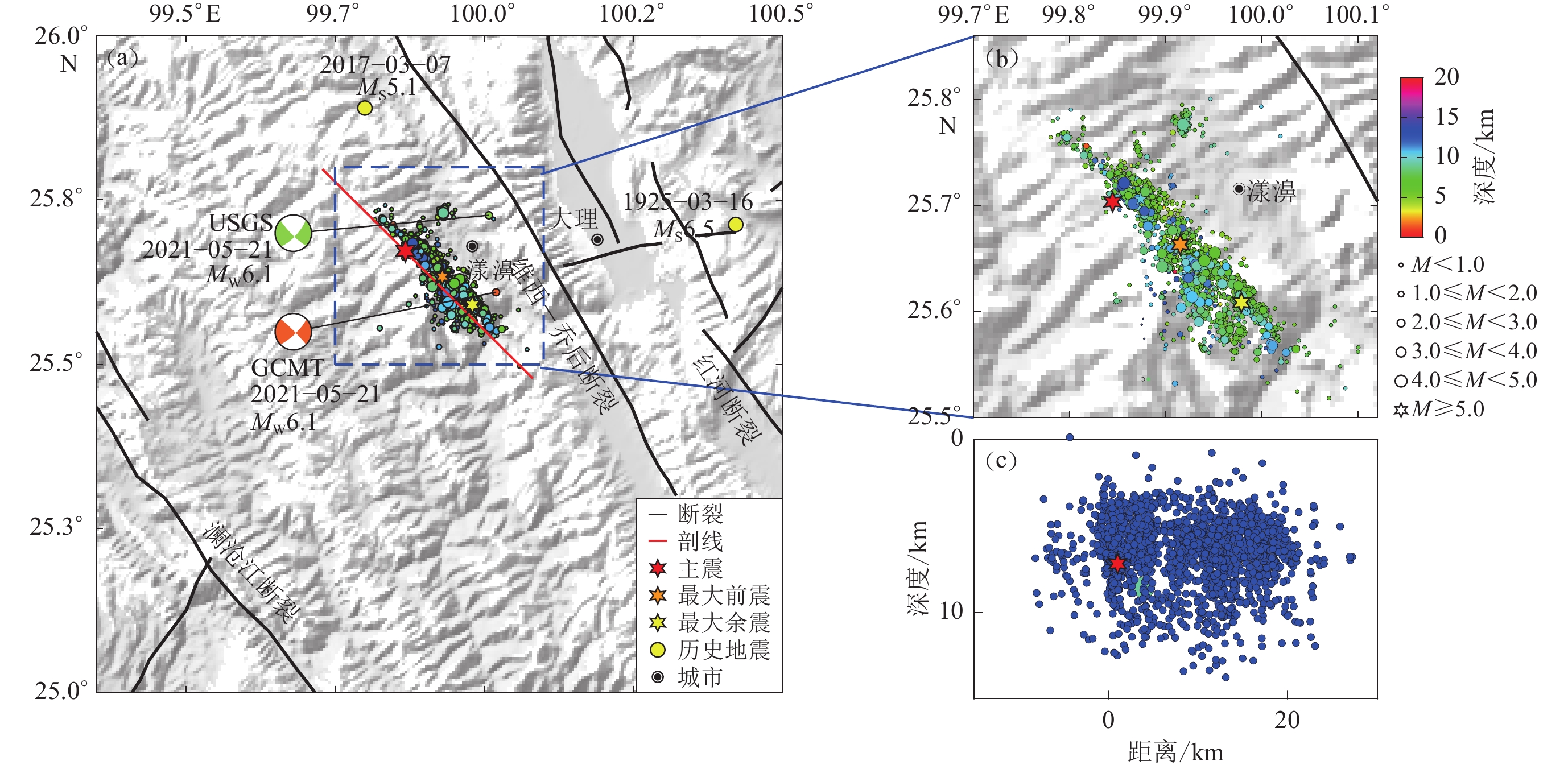
据中国地震台网测定,2021年5月21日21时48分在云南大理白族自治州漾濞县发生MS6.4地震,震中位置为(25.67°N,99.87°E),震源深度为8 km。国外地震研究机构USGS (United States Geological Survey)和GCMT (Global Centroid-Moment-Tensor Project)给出的震源深度分别为15 km和9 km。此次MS6.4地震发生在川滇地块的西南边界,震中距漾濞县城9 km,距大理市37 km。震中附近断裂众多,构造复杂,主要断裂为维西—乔后断裂和红河断裂(图1)。维西—乔后断裂西起维西县西北,在巍山以南与红河断裂带相接,是一条全长约280 km的右旋走滑型断裂,其总体走向呈NNW 向(常祖峰等,2016)。沿该断裂曾发生过1948年马登M6.25地震和2017年云南漾濞M5.1震群(潘睿等,2019)。震中东南的红河断裂是青藏高原东南缘一条走向NW的边界断裂带,分为北、中、南三段,全长1 000 km,其主要以右旋走滑运动为主。从地震记录来看,红河断裂震区附近曾发生过1652年弥渡M7.0地震和1925年大理M7.0地震(杨智娴等,2004)。根据震源机制解、地震波形反演及发震断层构造分析显示,该次地震为右旋走滑型地震,其发震断层为维西—乔后断裂的一条长约30 km的NW向平行伴生断裂,该断裂走向310°—320° (李传友等,2021;Wu et al,2011)。
![]() 图 1 云南漾濞MS6.4地震震中区构造背景(a)、地震序列空间分布(b)及剖面上的投影(c)Figure 1. Tectonic setting (a) of the epicentral area and spatial distribution (b) for Yunnan Yangbi MS6.4 earthquake sequence and its projection on profile (c)
图 1 云南漾濞MS6.4地震震中区构造背景(a)、地震序列空间分布(b)及剖面上的投影(c)Figure 1. Tectonic setting (a) of the epicentral area and spatial distribution (b) for Yunnan Yangbi MS6.4 earthquake sequence and its projection on profile (c)云南漾濞MS6.4地震属于前震-主震-余震型地震,主震前后发生多次M3.0以上地震。截至2021年5月26日,云南地震台网共记录到M≥0地震2 426次,其中,0≤ML<2.0地震1 492次,2.0≤ML<3.0地震383次,3.0≤ML<4.0地震67次,4.0≤ML<5.0地震21次,5.0≤ML<6.0地震5次(龙锋等,2021)。地震序列沿NW−SE展布,距离维西—乔后断裂3—10 km,呈现NW窄,SE宽的空间分布特征。地震密集区长约20 km,宽约5 km,主要分布在主震东南侧。地震震源深度集中分布在4—10 km,属于浅源型地震,破坏性较大。主震NE侧10 km处出现一个长约5 km的小震丛集区,总体呈NE−SW展布,与余震密集区主干序列垂直。最大前震(MS5.6)发生于21日21时21分25秒,位于地震序列主干中段,距离主震震中6 km。21日22时31分10秒于主震SE侧,距主震震中约15 km处发生最大余震,震级为MS5.3。
一次大地震发生后,其震源断裂错动引起应力场变化从而改变区域地震的活动性,这类影响称为应力触发,主要分为静态应力触发、黏弹性应力触发和动态应力触发三类(Kilb et al,2000;许才军等,2018)。对应力触发的研究工作是从静态应力触发开始的,始于上世纪60—80年代,经过多年的探索和研究,地震静态应力触发研究已经取得了很多成果,并得到了一些很有意义的结论(Reasenberg,Simpson,1992;Stein et al,1994;Pollitz,Sacks,1997;Toda et al,1998;缪淼,朱守彪,2013;盛书中等,2015;赵立波等,2016):正的库仑应力变化能促进断层的破裂,从而触发地震;反之,负的库仑应力变化抑制断层破裂,发生地震的可能性降低。1992年,美国加州兰德斯发生MW7.3地震,Kilb等(2000)同时计算兰德斯地震激发的静态应力和动态应力,对比发现动态应力能更好地解释地震发生率的变化,特别是地震活动率变化呈现的空间分布不对称性与动态库仑应力的空间分布不对称性之间有很好的一致性。自此,学者们开始对动态应力触发地震开展了一系列的研究(Hill et al,1993;Cotton,Coutant,1997;Brodsky et al,2000;Mohamad et al,2000;Wu et al,2011;冀战波等,2014;王琼等,2016)。大量的已有研究成果表明,动态库仑破裂应力变化具有非对称性而能更好地解释震后地震活动的变化,弥补了静态应力触发在解释震后余震的分布等方面存在的矛盾,即有的余震不仅没有发生在正的库仑破裂应力区,却发生在负的库仑破裂应力区。另一方面,静态应力受距离限制大,一般随着离发震断层距离倒数的3次方而迅速衰减(Steacy et al,2005)。随着距离地震破裂越来越远,静态应力作用越来越小,而由地震波产生的动态应力随距离衰减相对较慢,且其变化远远大于静态应力变化,因而能够更好地解释主震发生后余震区的小震活动以及远场区域的中小地震活动。因此,开展大地震对后续地震的动态应力触发研究受到广泛关注,研究云南漾濞MS6.4地震震后对后续余震活动的触发影响具有重要意义。
针对本次地震序的列分布特点,本文首先基于有限断层反演方法获取比较可靠的破裂过程参数,结合震源机制解参数构建主震可靠的震源模型,然后基于离散波数法计算漾濞MS6.4地震断层破裂在近场产生的库仑破裂应力变化,定量研究MS6.4地震对近场余震活动的动态应力触发作用,从而探讨MS6.4地震对余震区活动特征的影响。
1. 研究区域和模型参数
云南漾濞MS6.4地震发生后,国外地震研究机构USGS和GCMT给出了主震的震源机制解,龙锋等(2021)采用CAP波形反演方法得到主震震源机制解,具体参数见表1。以USGS震源参数为基础,假设震源为一个以有限速度扩展的双侧破裂走滑断层,断层长度为40 km,宽度为18 km,将震源发震断层以2 km为间隔分解成9×20个小单元面,共计180个子断层。以IRIS数据中心的地震数据资料为基础,选取其中信噪比较高且沿方位角分布比较均匀的14个远场P波波形(30°
$<\varDelta < $ 90°)数据进行平面有限断层的破裂过程反演。台站分布及其拟合波形见图2a,观测波形与理论波形的拟合率为67%。得到的破裂过程反演结果见图2b。表 1 云南漾濞MS6.4地震震源参数Table 1. Focal mechanism parameters of the Yunnan Yangbi MS6.4 earthquake发震日期 震中位置 MW 深度/km 节面Ⅰ 节面Ⅱ 来源 年-月-日 北纬/° 东经/° 走向/° 倾角/° 滑动角/° 走向/° 倾角/° 滑动角/° 25.61 100.02 6.1 15.0 46 78 4 315 86 168 GCMT (2021) 2021-05-21 25.73 100.01 6.1 9.0 135 82 −165 43 75 −9 USGS (2021) 25.69 99.88 5.9 7.8 135 75 −168 42 78 −15 重定位(龙锋等,2021) ![]() 图 2 台站分布和P波垂向位移理论图(红线)与观测波形(黑线)的拟合情况(a)以及每2秒破裂快照(b)Figure 2. Station distribution and the fitting of P-wave vertical displacement theoretical graph (red line) and observed waveform (black line) (a) and snapshot shown every 2 s (b)
图 2 台站分布和P波垂向位移理论图(红线)与观测波形(黑线)的拟合情况(a)以及每2秒破裂快照(b)Figure 2. Station distribution and the fitting of P-wave vertical displacement theoretical graph (red line) and observed waveform (black line) (a) and snapshot shown every 2 s (b)研究区域的地壳结构选取非均匀弹性半无限空间,不同的地壳深度选取不同的P波速度和S波速度,地壳密度取值相同,P波和S波Q值也相同,速度模型参考了吴建平等(2004)对云南地区人工地震折射和区域地震波形反演得到的速度结果(表2)。
表 2 云南漾濞MS6.4地震震源附近地壳分层模型Table 2. Crustal layered model near the seismic source of the Yunnan Yangbi MS6.4 earthquake深度/km vP/(km·s−1) vS/(km·s−1) 地壳密度/(g·cm−3) QP QS 0 7.75 4.47 3.37 600 300 4 4.85 2.80 3.37 600 300 16 6.25 3.61 3.37 600 300 22 6.40 3.70 3.37 600 300 以有限断层破裂反演结果为基础,选取(25.2°—25.9°N,99.5°—100.2°E)为近场研究区域,以0.07°×0.07°为步长划分研究区,共获得近场研究区121个接收点。根据反演结果,滑动振幅取0.5 m,破裂持续时间取20 s,上升时间取破裂持续时间的1/10 (Meyer,Kearnes,2013),即2 s。结合研究区域的地壳结构和主震的震源机制解,研究主震在近场区域产生的动态库仑破裂应力的时空演化过程,从而讨论主震对后续地震活动的应力触发作用。
2. 原理与方法
基于反射率(Muller,1985)和格林函数(Bouchon,1981)在轴对称介质中的离散波数法(discrete wave-number method,缩写为DWN)(Bouchon,2003)可以通过计算震源断层在任一接收点处产生的地震波位移求得应变和应力,得到接收点处同时包含了动态和静态库仑破裂应力变化的完全库仑破裂应力时空演化过程。而地震的应力触发是指主震对后续地震活动性的影响,所以主震的各种参数(震源机制解和破裂过程)都会对最终计算的动态库仑破裂应力产生影响,故在计算动态应力前需获得比较可靠的主震参数。因此,本文讨论动态库仑破裂应力触发影响时主要包括如下几个步骤:
1) 基于有限断层方法反演主震破裂过程,获取主震发生时的位错量、总破裂时间和破裂速度等。利用远震台站地震波数据,根据震源断层几何参数和地壳速度模型基于频率-波数法构建格林函数,引进拉普拉斯平滑约束作为约束条件,采用多时窗反演方法(Hartzell,Heaton,1983)对主震破裂过程进行反演。
2) 根据步骤1获得的主震破裂模型参数,基于DWN方法计算主震破裂在某深度介质平面各接收点产生的地震波位移μi(x,t)。其原理是用复合源代替单一稳定源稳定辐射柱状波,在二维情况下,其位移或应力表示为:
$$ G ( x, {\textit{z}}; \omega ) = \frac{{2\pi }}{L}\sum\limits_{n = - \infty }^\infty {f ( {k_n}, {\textit{z}} ) {{\rm{e}}^{ - {\rm{i}}{k_n}x}}} {,} $$ (1) 式中:ω为角频率;k为水平波数,kn=2πn/L,L为周期源的间隔。
3) 将地震波位移进行弹性动力性转换得到动态库仑破裂应力变化。首先应用差分原理计算出应变分量,再由胡克定律由应变转换为应力,得到主震地震波在各接收点产生的应力分量。在此基础上,由柯西公式得到投影断层面上的动态应力变化矢量,分别投影到断层面的法线方向和滑动方向单位矢量上,得到正应力变化∆σ(x,t)和切应力变化∆τ(x,t),则动态库仑破裂应力(Coulomb failure stress,缩写为∆CFS)变化为:
$$ \Delta {\rm{CFS}} ( x, t ) = \Delta \tau ( x, t ) + {\mu '}\Delta \sigma ( x, t ) {,} $$ (2) 式中,
$\mu ' $ 为视摩擦系数,取0.5。当库仑破裂应力变化为正值时,可促使断层发生断裂,使地震活动性增加。一般来说,当动态库仑破裂应力变化最大正值大于动态触发阈值0.1 MPa (Kilb et al,2000;郝平等,2006),则认为动态应力有可能触发地震;当稳定值即静态库仑破裂应力值高于静态触发阈值0.01 MPa (Harris,1998;缪淼,朱守彪,2016),则认为静态应力有可能触发地震。
3. 结果分析
3.1 动态库仑破裂应力对近场后续地震活动的影响
主震发生后,静态和动态库仑破裂应力均会对近场区域的地震活动性产生影响。为探究云南MS6.4地震产生的静态库仑破裂应力对后续余震活动影响较大还是动态库仑破裂应力影响较大,本文首先根据Okada (1992)弹性半空间位错理论,通过应力、应变的本构关系,假设空间中接收断层的参数与主震一致,选择重定位后的主震节面Ⅰ的参数作为接收断层参数,计算了震源深度7.8 km上的静态库仑破裂应力变化,得到结果如图3a所示。从图中可以看出,静态应力呈现四象限对称分布,余震的分布趋势则是大致沿NW−SE展布,余震位于静态库仑破裂应力正值区域的比例为43%。
![]() 图 3 云南漾濞MS6.4地震静态应力变化(a)和地震序列密度分布及MS4.0以上余震震源机制(b)Figure 3. Static stress change of the Yunnan Yangbi MS6.4 earthquake (a) and density distribution of the earthquake sequence and focal mechanisms of aftershocks above MS4.0
图 3 云南漾濞MS6.4地震静态应力变化(a)和地震序列密度分布及MS4.0以上余震震源机制(b)Figure 3. Static stress change of the Yunnan Yangbi MS6.4 earthquake (a) and density distribution of the earthquake sequence and focal mechanisms of aftershocks above MS4.0为详细展示漾濞MS6.4地震序列的空间分布细节,以0.07°×0.07°的步长划分空间节点,以空间节点1 km范围内的地震频数lgN作为地震密度,得到密度分布图(图3b)。整个余震序列分布呈现集中-稀疏-集中的趋势。在主震北东方向出现一个小型余震丛集,其分布呈NE-SW分布,垂直于余震主干序列。
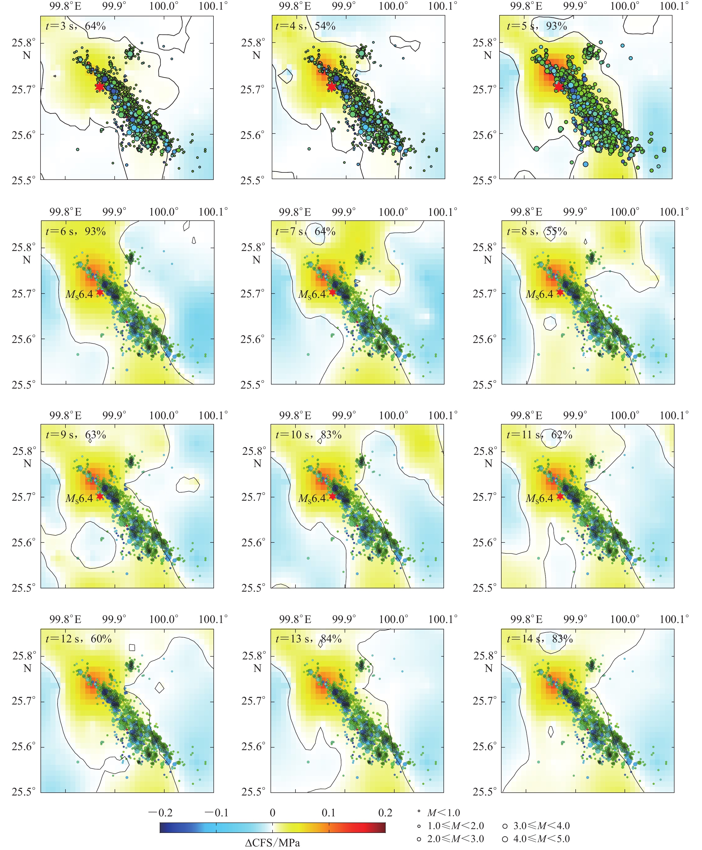
以重定位后的主震节面I的参数作为接收断层参数,计算得到云南漾濞MS6.4地震近场产生的动态库仑破裂应力演化的空间图像并统计余震位于动态应力正值区域的比例(图4)。作图时有意缩小图幅范围,以便突出应力变化与余震分布的关系。从图中可以看到,地震发生后的前10 s,动态库仑破裂应力变化的空间分布图像演化较快,正值区域主要分布在MS6.4地震的SE侧,并逐渐向NW扩大。20 s后,动态库仑破裂应力的空间分布图像基本稳定,说明已基本进入静态库仑破裂应力变化阶段,余震位于动态应力正值区域的比例为63%。余震主要分布在动态应力为正的区域,表明主震产生的库仑破裂应力有利于促进该区域余震的发生。∆CFS在第5 s左右达到最大值,最大值为0.15 Mpa,位于(99.85°E,25.69°N),离主震震中约3 km,此时余震位于动态库仑破裂应力正值区域的比例最大,为93%。结合密度图和∆CFS的动态演化图可以看出,主震震中附近及NW侧∆CFS值较大,余震分布更密集,而地震序列中段∆CFS值较小,余震分布则相对稀疏,说明当∆CFS为正时,其大小分布与整个余震序列空间散落的疏密程度相对应,即∆CFS值越大,对地震的触发影响越大。
![]() 图 4 ∆CFS动态演化图中百分数表示余震位于动态库仑破裂应力正值区域的比例Figure 4. Dynamic evolution of ∆CFSThe percentage in the figure shows the proportion of aftershocks in the positive value area of dynamic Coulomb stress
图 4 ∆CFS动态演化图中百分数表示余震位于动态库仑破裂应力正值区域的比例Figure 4. Dynamic evolution of ∆CFSThe percentage in the figure shows the proportion of aftershocks in the positive value area of dynamic Coulomb stress![]() 图 4 ∆CFS动态演化图中百分数表示余震位于动态库仑破裂应力正值区域的比例Figure 4. Dynamic evolution of ∆CFSThe percentage in the figure shows the proportion of aftershocks in the positive value area of dynamic Coulomb stress
图 4 ∆CFS动态演化图中百分数表示余震位于动态库仑破裂应力正值区域的比例Figure 4. Dynamic evolution of ∆CFSThe percentage in the figure shows the proportion of aftershocks in the positive value area of dynamic Coulomb stress在主震震中NE方向10 km处出现小型余震丛集区,该区域位于静态库仑破裂应力的负值区域,而在动态应力演化图上,该区域从主震后第3 s起,便几乎一直处于动态库仑破裂应力为正的区域,表明该区域的小震丛集现象可能是由主震产生的动态应力触发作用导致的。
根据云南MS6.4地震破裂反演结果(图2b),本次地震破裂在断层面的分布比较集中,破裂主要发生在主震NW侧3 km附近,整个地震破裂过程持续了20 s,主要集中在前15 s。破裂自起始破裂点开始,前2 s为破裂的初始阶段,滑动范围和量级都很小;4—6 s,破裂沿走向方向在浅层传播;自8 s开始,破裂沿倾角向下延伸;8—10 s,震源上方和下方的破裂继续传播;其后自12 s开始,随着破裂的持续延伸,逐渐形成了以震源为中心的破裂区。滑移峰值出现在地震发生后的第6 s,断层滑动量约为0.059 m。从第15 s开始,滑动量又开始逐渐减小。图4显示:4 s开始主震SE方向出现大范围动态库仑破裂应力变化正值区域;5—6 s,余震位于动态库仑破裂应力正值区域的比例为93%,是整个演化过程中的最大值;20 s后,动态应力正值区域分布区域稳定。MS6.4地震破裂过程结果与其在不同时刻产生的动态库仑破裂应力变化结果较为一致。
3.2 近场余震活动的动态应力触发
为定量分析MS6.4地震对近场余震区的应力触发作用,分别计算了主震震后MS≥4.0余震震源处的动态库仑应力变化量。以龙锋等(2021)对MS6.4漾濞地震序列MS4.0以上事件CAP波形反演方法得到的震源机制解为基础(图3b),计算震源机制解节面Ⅰ的动态应力变化图(图5),分析MS6.4地震对MS≥4.0余震的应力触发影响(表3)。主震震后一周内MS≥4.0的8次余震的接收点均受到动态库仑破裂应力的触发作用。其中动态应力峰值较大的地震为②—⑥号地震,②,③,④号地震位于地震序列SE侧,⑤,⑥地震位于主震震中附近。静态应力对①,⑥,⑦号地震有一定的触发作用,对③号和⑧号地震可能有触发作用。
![]() 表 3 主震对MS≥4.0余震应力触发情况Table 3. The stress trigger of the main shock to MS≥4.0 aftershocks
表 3 主震对MS≥4.0余震应力触发情况Table 3. The stress trigger of the main shock to MS≥4.0 aftershocks地震序号 与主震震中的
距离/km开始变化
时间/s达到峰值
时间/s∆CFS峰值
/MPa趋于稳定
时间/s稳定值
/MPa应力触发 1 8.67 2.0 3.7 0.13 13 0.09 动态、静态应力触发 2 12.68 1.7 5.3 0.83 16 −0.001 动态应力触发 3 13.49 2.0 5.3 0.47 13 0.01 动态应力触发,静态应力可能触发 4 13.49 1.9 5.7 0.27 14 −0.02 动态应力触发 5 2.22 3.0 3.5 0.39 动态应力触发 6 1.00 1.8 8.4 0.50 12 0.48 动态、静态应力触发 7 8.98 2.0 7.4 0.12 11 0.09 动态、静态应力触发 8 11.17 5.0 7.5 0.18 13 0.02 动态应力触发,静态应力可能触发 4. 讨论与结论
为讨论云南漾濞MS6.4地震产生的动态库仑破裂应力对后续地震活动的影响,本文首先利用远震台站波形数据,基于有限断层反演方法获得比较可靠的破裂过程参数,然后结合较为准确的震源机制解参数和介质模型参数,基于离散波数法计算了云南漾濞MS6.4地震断层破裂在近场产生的库仑破裂应力变化,讨论了云南漾濞MS6.4地震对近场余震活动的动态应力触发影响。
主震产生的动态库仑破裂应力在3 s左右开始变化,前10 s变化较快,20 s以后趋于稳定。余震位于动态库仑破裂应力正值区域的比例在5—6 s达到峰值。动态破裂应力正值较大区域主要分布在震中NW侧,这与主震震源破裂特征反演结果一致。其大小分布与整个余震序列空间散落的疏密程度有较好的相关性,主震震中附近及NW侧∆CFS值较大,余震分布更密集,而地震序列中段∆CFS值较小,余震分布则相对稀疏。
结合云南漾濞MS6.4地震在近场产生的静态库仑破裂应力(图3a)和在不同时刻产生的近场库仑破裂应力演化图(图4),MS6.4地震序列主要分布在库仑应力变化为正的区域,说明动态应力和静态应力对区域内余震活动具有一定的促进作用,是造成近场地震活动性增加的可能原因。而相比静态应力,余震发生在静态应力正值区域的比例为42%,发生在动态应力(稳定后)正值区域的比例为63%,比例提高了21%,说明余震发生位置与静态应力变化正值区域相关性不大,与动态库仑应力变化的正负区域有更好的一致性,从动态应力的角度能更好地解释震后余震分布的空间特征。
主震产生的动态库仑破裂应力变化有利于主震震中北东方向10 km处的余震丛集活动,但静态应力变化不利于该区的余震活动。该区域处于静态应力负值区域,动态应力正值区域。动态应力变化可能诱发除主震断层以外其它断层的活动,这可能是该区域余震活动密集的主要原因。静态应力变化对该区域的余震活动具有一定的抑制作用,这可能是该区的余震活动水平不高的原因。综合分析认为,针对漾濞MS6.4地震序列,该区域的余震活动可能是由动态应力起主导作用。
在计算地震应力时,存在一些不确定因素和误差影响。首先,采用远震P波反演主震破裂过程,可能存在分辨率不足,可加入近场波形数据以及一些大地动力学观测资料如GPS等进行联合反演,那么对震源破裂过程的时空过程将更为细致,分辨率也将大大提高。其次,由于缺乏本地区精细的三维速度模型等参数,故本文建立的模型是基于前人的研究成果,采用的是比较简单的弹性半空间模型。而在实际中,由于地球介质的不均匀结构分布,会导致对应力的计算产生一定的影响。因此,考虑使用趋于真实的介质模型是后续改进的方向。最后,本文采用主震的震源机制作为整个研究区域的接收断层参数,不同的接收断层参数对库仑应力场的大小分布会产生一定的影响。而在定量计算主震对余震产生的动态应力变化时,以余震发震断层面的震源机制解作为接收断层参数会减小一定的误差。但由于M4.0地震震级相对较小,受资料限制,无法确认余震的发震断层面,存在一定的不确定性。与此同时,余震的定位误差、后续余震的分布不均匀以及对背景应力场的认识有限等都会对库仑应力的结果与分析产生一定的影响,但根据动态应力演化过程定性研究主震产生的动态应力对后续余震活动性的影响,能够为后续可能发生余震的区域的预测提供一定的参考。
-
![]()
图 3 云南漾濞MS6.4地震静态应力变化(a)和地震序列密度分布及MS4.0以上余震震源机制(b)
Figure 3. Static stress change of the Yunnan Yangbi MS6.4 earthquake (a) and density distribution of the earthquake sequence and focal mechanisms of aftershocks above MS4.0
![]()
图 1 云南漾濞MS6.4地震震中区构造背景(a)、地震序列空间分布(b)及剖面上的投影(c)
Figure 1. Tectonic setting (a) of the epicentral area and spatial distribution (b) for Yunnan Yangbi MS6.4 earthquake sequence and its projection on profile (c)
![]()
图 2 台站分布和P波垂向位移理论图(红线)与观测波形(黑线)的拟合情况(a)以及每2秒破裂快照(b)
Figure 2. Station distribution and the fitting of P-wave vertical displacement theoretical graph (red line) and observed waveform (black line) (a) and snapshot shown every 2 s (b)
![]()
图 4 ∆CFS动态演化
图中百分数表示余震位于动态库仑破裂应力正值区域的比例
Figure 4. Dynamic evolution of ∆CFS
The percentage in the figure shows the proportion of aftershocks in the positive value area of dynamic Coulomb stress
![]()
图 4 ∆CFS动态演化
图中百分数表示余震位于动态库仑破裂应力正值区域的比例
Figure 4. Dynamic evolution of ∆CFS
The percentage in the figure shows the proportion of aftershocks in the positive value area of dynamic Coulomb stress
![]()
表 1 云南漾濞MS6.4地震震源参数
Table 1 Focal mechanism parameters of the Yunnan Yangbi MS6.4 earthquake
发震日期 震中位置 MW 深度/km 节面Ⅰ 节面Ⅱ 来源 年-月-日 北纬/° 东经/° 走向/° 倾角/° 滑动角/° 走向/° 倾角/° 滑动角/° 25.61 100.02 6.1 15.0 46 78 4 315 86 168 GCMT (2021) 2021-05-21 25.73 100.01 6.1 9.0 135 82 −165 43 75 −9 USGS (2021) 25.69 99.88 5.9 7.8 135 75 −168 42 78 −15 重定位(龙锋等,2021)  下载: 导出CSV
表 2 云南漾濞MS6.4地震震源附近地壳分层模型
Table 2 Crustal layered model near the seismic source of the Yunnan Yangbi MS6.4 earthquake
深度/km vP/(km·s−1) vS/(km·s−1) 地壳密度/(g·cm−3) QP QS 0 7.75 4.47 3.37 600 300 4 4.85 2.80 3.37 600 300 16 6.25 3.61 3.37 600 300 22 6.40 3.70 3.37 600 300
下载: 导出CSV
表 3 主震对MS≥4.0余震应力触发情况
Table 3 The stress trigger of the main shock to MS≥4.0 aftershocks
地震序号 与主震震中的
距离/km开始变化
时间/s达到峰值
时间/s∆CFS峰值
/MPa趋于稳定
时间/s稳定值
/MPa应力触发 1 8.67 2.0 3.7 0.13 13 0.09 动态、静态应力触发 2 12.68 1.7 5.3 0.83 16 −0.001 动态应力触发 3 13.49 2.0 5.3 0.47 13 0.01 动态应力触发,静态应力可能触发 4 13.49 1.9 5.7 0.27 14 −0.02 动态应力触发 5 2.22 3.0 3.5 0.39 动态应力触发 6 1.00 1.8 8.4 0.50 12 0.48 动态、静态应力触发 7 8.98 2.0 7.4 0.12 11 0.09 动态、静态应力触发 8 11.17 5.0 7.5 0.18 13 0.02 动态应力触发,静态应力可能触发
下载: 导出CSV
-
常祖峰,常昊,李鉴林,代博洋,周青云,朱家龙,罗宗其. 2016. 维西—乔后断裂南段正断层活动特征[J]. 地震研究,39(4):579–586. doi: 10.3969/j.issn.1000-0666.2016.04.007 Chang Z F,Chang H,Li J L,Dai B Y,Zhou Q Y,Zhu J L,Luo Z Q. 2016. The characteristic of active normal faulting of the southern segment of Weixi−Qiaohou fault[J]. Journal of Seismological Research,39(4):579–586 (in Chinese).
郝平,刘杰,韩竹军,傅征祥. 2006. 印尼MS8.7地震对中国大陆3次后续中强地震的动应力触发研究[J]. 地震,26(3):26–36. Hao P,Liu J,Han Z J,Fu Z X. 2006. Dynamic stress triggering of three subsequent moderately strong earthquakes in China’s mainland following the Indonesia MS8.7 earthquake[J]. Earthquake,26(3):26–36 (in Chinese).
冀战波,王琼,王海涛,解朝娣. 2014. 2008年新疆于田MS7.3地震对后续地震的完全库仑应力触发作用[J]. 地震学报,36(6):997–1009. Ji Z B,Wang Q,Wang H T,Xie C D. 2014. Impact of complete Coulomb failure stress changes of the 2008 Xinjiang Yutian MS7.3 earthquake on the subsequent earthquakes[J]. Acta Seismologica Sinica,36(6):997–1009 (in Chinese).
李传友,张金玉,王伟,孙凯,单新建. 2021. 2021年云南漾濞 6.4 级地震发震构造分析[J]. 地震地质,43(3):706–721. doi: 10.3969/j.issn.0253-4967.2021.03.015 Li C Y,Zhang J Y,Wang W,Sun K,Shan X J. 2021. The seismogenic fault of the 2021 Yunnan Yangbi MS6.4 earthquake[J]. Seismology and Geology,43(3):706–721 (in Chinese).
龙锋,祁玉萍,易桂喜,吴微微,王光明,赵小艳,彭关灵. 2021. 2021年5月21日云南漾濞MS6.4地震序列重新定位与发震构造分析[J]. 地球物理学报,64(8):2631–2646. Long F,Qi Y P ,Yi G X,Wu W W,Wang G M,Zhao X Y,Peng G L. 2021. Relocation of the MS6.4 Yangbi earthquake sequence on May 21,2021 in Yunnan Province and its seismogenic structure analysis[J]. Chinese Journal of Geophysics,64(8):2631–2646 (in Chinese).
缪淼,朱守彪. 2013. 2013年芦山MS7.0地震产生的静态库仑应力变化及其对余震空间分布的影响[J]. 地震学报,35(5):619–631. Miao M,Zhu S B. 2013. The static Coulomb stress change of the 2013 Lushan MS7.0 earthquake and its impact on the spatial distribution of aftershocks[J]. Acta Seismologica Sinica,35(5):619–631 (in Chinese).
缪淼,朱守彪. 2016. 2014年鲁甸地震(MS=6.5)静态库仑应力变化及其影响[J]. 地震地质,38(1):169–181. Miao M ,Zhu S B. 2016. The static Coulomb stress change of the 2014 Ludian earthquake and its influence on the aftershocks and surrounding faults[J]. Seismology and Geology,38(1):169–181 (in Chinese).
潘睿,姜金钟,付虹,李姣. 2019. 2017年云南漾濞MS5.1及MS4.8地震震源机制解和震源深度测定[J]. 地震研究,42(3):338–348. doi: 10.3969/j.issn.1000-0666.2019.03.005 Pan R,Jiang J Z,Fu H,Li J. 2019. Focal mechanism and focal depth determination of Yunnan Yangbi MS5.1 and MS4.8 earthquakes in 2017[J]. Journal of Seismological Research,42(3):338–348 (in Chinese).
盛书中,万永革,蒋长胜,卜玉菲. 2015. 2015年尼泊尔MS8.1强震对中国大陆静态应力触发影响的初探[J]. 地球物理学报,58(5):1834–1842. Sheng S Z,Wan Y G,Jiang C S,Bu Y F. 2015. Preliminary study on the static stress triggering effects on China mainland with the 2015 Nepal MS8.1 earthquake[J]. Chinese Journal Of Geophysics,58(5):1834–1842 (in Chinese).
王琼,解朝娣,冀战波,刘建明. 2016. 2014年于田MS7.3地震对后续余震和远场小震活动的动态应力触发[J]. 地球物理学报,59(4):1383–1393. Wang Q,Xie C D,Ji Z B,Liu J M. 2016. Dynamically triggered aftershock activity and far-field microearthquakes following the 2014 MS7.3 Yutian,Xinjiang earthquake[J]. Chinese Journal of Geophysics,59(4):1383–1393 (in Chinese).
吴建平,明跃红,王椿镛. 2004. 云南地区中小地震震源机制及构造应力场研究[J]. 地震学报,26(5):457–465. doi: 10.3321/j.issn:0253-3782.2004.05.001 Wu J P,Ming Y H,Wang C Y. 2004. Source mechanism of small-to-moderate earthquakes and tectonic stress field in Yunnan Province[J]. Acta Seismologica Sinica,26(5):457–465 (in Chinese).
许才军,汪建军,熊维. 2018. 地震应力触发回顾与展望[J]. 武汉大学学报信息科学版,43(12):2085–2092. Xu C J,Wang J J,Xiong W. 2018. Retrospection and perspective for earthquake stress triggering[J]. Geomatics and Information Science of Wuhan University,43(12):2085–2092 (in Chinese).
杨智娴,于湘伟,郑月军,陈运泰,倪晓晞,Chan W. 2004. 中国中西部地区地震的重新定位和三维地壳速度结构[J]. 地震学报,26(1):19–19. doi: 10.3321/j.issn:0253-3782.2004.01.003 Yang Z X,Yu X W,Zheng Y J,Chen Y T,Ni X X,Chan W. 2004. Earthquake relocation and 3-dimensional crustal structure of P-wave velocity in central-western China[J]. Acta Seismologica Sinica,26(1):19 (in Chinese).
赵立波,赵连锋,谢小碧,曹俊兴,姚振兴. 2016. 2014年2月12日新疆于田MW7.0地震源区静态库仑应力变化和地震活动率[J]. 地球物理学报,59(10):3732–3743. Zhao L B,Zhao L F,Xie X B,Cao J X,Yao Z X. 2016. Static Coulomb stress changes and seismicity rate in the source region of the 12 February,2014 MW7.0 Yutian earthquake in Xinjiang,China[J]. Chinese Journal of Geophysics,59(10):3732–3743 (in Chinese).
Bouchon M. 1981. A simple method to calculate Green’s functions for elastic layered media[J]. Bull Seism Soc Am,71(4):959–971.
Bouchon M. 2003. A review of the discrete wavenumber method[J]. Pure Appl Geophys,160(3):445–465.
Brodsky E E,Karakostas V,Kanamori H. 2000. A new observation of dynamically triggered regional seismicity:Earthquakes in Greece following the August 1999 Izmit,Turkey earthquake[J]. Geophys Res Lett,27(1):2741–2744.
Cotton F,Coutant O. 1997. Dynamic stress variations due to shear faults in a plane-layered medium[J]. Geophys J Int,128(3):676–688.
GCMT. 2021. 202105211348A Yunnan, China[DB/OL]. [2021-05-28]. https://www.globalcmt.org/.
Harris R A. 1998. Introduction to special section:Stress triggers,stress shadows,and implications for seismic hazard[J]. J Geophys Res:Solid Earth,103(B10):24347–24358. doi: 10.1029/98JB01576
Hartzell S H,Heaton T H. 1983. Inversion of strong ground motion and teleseismic waveform data for the fault rupture history of the 1979 Imperial Valley,California,earthquake[J]. Bull Seism Soc Am,73(6A):1553–1583.
Hill D P,Reasenberg P A,Michael A,Arabaz W J,Beroza G,Brumbaugh D,Brune J N,Castro R,Davis S,Depolo D,Ellsworth W L,Gomberg J,Harmsen S,House L,Jackson S M,Johnston M J S,Jones L,Keller R,Malone S,Munguia L,Nava S,Pechmann J C,Sanford A,Simpson R W,Smith R B,Stark M,Stickney M,Vidal A,Walter S,Wong V,Zollweg J. 1993. Seismicity remotely triggered by the magnitude 7.3 Landers,California,earthquake[J]. Science,260(5114):1617–1623. doi: 10.1126/science.260.5114.1617
Kilb D,Gomberg J,Bodin P. 2000. Triggering of earthquake aftershocks by dynamic stresses[J]. Nature,408:570–574.
Meyer M,Kearnes K. 2013. Introduction to special section:Intermediaries between science,policy and the market[J]. Sci Public Policy,40(4):423–429.
Mohamad R,Darkal A N,Seber D,Sandvol E,Gocuez F,Barazangi M. 2000. Remote earthquake triggering along the Dead Sea fault in Syria following the 1995 Gulf of Aqaba earthquake (MS=7.3)[J]. Seismological Research Letters,71(1):47–52. doi: 10.1785/gssrl.71.1.47
Muller G. 1985. The reflectivity method:A tutorial[J]. J Geophys Int,58(1/2/3):153–174.
Okada Y. 1992. Internal deformation due to shear and tensile faults in a half-space[J]. Bull Seism Soc Am,82(2):1018–1040. doi: 10.1785/BSSA0820021018
Pollitz F F,Sacks I S. 1997. The 1995 Kobe,Japan,earthquake:A long-delayed aftershock of the offshore 1944 Tonankai and 1946 Nankaido earthquakes[J]. Bull Seisml Soc Am,87(1):1–10.
Reasenberg P A,Simpson R W. 1992. Response of regional seismicity to the static stress change produced by the Loma-Prieta earthquake[J]. Science,255(5052):1687–1690. doi: 10.1126/science.255.5052.1687
Steacy S,Nalbant S S,Mccloskey J,Nostro C,Scotti O,Baumont D. 2005. Onto what planes should Coulomb stress perturbations be resolved?[J]. J Geophys Res,110(B5):B05S15.
Stein R S,King G C,Lin J. 1994. Stress triggering of the 1994 M6.7 Northridge,California,earthquake by its predecessors[J]. Science,265(5177):1432–1435. doi: 10.1126/science.265.5177.1432
Toda S,Stein R S,Reasenberg P A,Dieterich J H,Yoshida A. 1998. Stress transferred by the 1995 MW6.9 Kobe,Japan,shock:Effect on aftershocks and future earthquake probabilities[J]. J Geophys Res:Solid Earth,103(B10):24543–24565. doi: 10.1029/98JB00765
USGS. 2021. M6.1: 25 km NW of Dali, China[DB/OL]. [2021-05-28]. https://earthquake.usgs.gov/earthquakes/eventpage/us7000e532/moment-tensor.
Wu C Q,Peng Z G,Wang W J,Chen Q F. 2011. Dynamic triggering of shallow earthquakes near Beijing,China[J]. Geophys J Int,185(3):1321–1334.


计量
- 文章访问数: 387
- HTML全文浏览量: 155
- PDF下载量: 129
