

Modification of fitting parameters in coherency model for spatial variation of seismic ground motion
-
摘要: 采用SMART-1台阵第5次和第45次地震的水平向分量加速度记录,首先计算了不同间距台站对的地震动空间相干函数;然后讨论了台站距离对相干函数拟合结果的影响,即某一特定距离的相干函数与所有不同距离的相干函数的拟合结果存在明显差异。为减小这一差异,提出了一种对各个不同距离的相干函数拟合参数进行二次回归的方法,并选用Loh相干函数模型进行了验证,最后给出了基于Loh相干函数模型的拟合参数的修正结果。结果表明本文提出的修正方法将大大提高相干函数模型中参数的拟合精度。
-
关键词:
- SMART-1 台阵 /
- 地震动空间相关性 /
- 相干函数 /
- 台站间距 /
- 参数拟合
Abstract: In this study, the horizontal component of the 5th and the 45th seismic records of the SMART-1 array were selected. Firstly the lagged coherencies of seismic ground motion of station pairs with different separation distances were calculated. Then the influence of station distance on the fitting of parameters of the coherency function model was discussed, that is, there were obvious differences between the fitting results of the coherency function of a certain distance and the coherency functions of all different distances. In order to reduce this deviation, a method of quadratic regression on the fitting parameters of the coherency of different distances was proposed, and the Loh coherency function model was selected for verifying the method. Finally, the correction results of the fitting parameters based on the Loh coherency function model were given. The results show that the correction method proposed in this paper will greatly improve the fitting accuracy of the parameters in the coherence function model. -
引言
产生地震动空间变化的原因多且复杂,与之密切相关的因素主要有震源性质(包括震源深度、断层的有限尺度和破裂方式)、传播途径和场地条件等(Abrahamson,1993;der Kiureghian,1996),而地震动的这种空间变化对生命线工程如大坝、大跨桥梁、高速铁路、地铁和地下管线等长、大结构的地震反应有很大影响(Park et al,2009;Chopra,Wang,2010;Bi et al,2013;Wu et al,2016;Li et al,2017;Liu,Gao,2018)。目前,研究地震动空间变化最常用的方法是相干函数法,各国研究人员提出了大量的描述地震动空间变化的相干函数模型(Zerva,2009),这些模型中的相干系数主要是基于高密度强震观测台网(台阵)的加速度记录统计拟合得到(Loh,1985;Harichandran,Vanmarcke,1986;Hao,1989;Abrahamson et al,1991;屈铁军等,1996;刘先明等,2004;李英民等,2013)。相干函数模型中的两个主要参数为频率f和台站间距离d。统计获得的所有相干函数模型均具有相同的变化规律,即随频率或距离的增大相干函数逐渐减小。在进行相干函数模型参数的拟合时,截止频率的取值对地震动空间相干函数统计结果有很大影响(丁海平等,2018),所以,不同相干函数模型基本给出了相应的频率使用范围。而由于研究地震动空间变化的强震台阵间台站距离d的变化范围较小(台站数量较少,且台站间的距离一般集中在数十米至数千米之间),因此对距离d的范围和不同的间距数量的选取也影响着相干函数的拟合结果(饶威波等, 2018)。例如,对应不同距离d的相干函数,按照假定的相干函数数学模型可以得到各自的拟合参数;而对所有不同距离的相干函数进行拟合,也可以得到一组统一的拟合参数。但是,根据某一特定距离的相干函数得到的拟合(参数)曲线,与根据所有不同距离的相干系数统一回归得到的该距离的相干函数拟合(参数)曲线是不一致的,有时甚至偏差较大。为了减小该偏差,本文拟提出一种修正方法,即对由不同距离得到的相干函数模型中的参数进行二次回归,得到一组针对距离的参数修正表达式,以期提高相干函数模型中参数的拟合精度,并以SMART-1台阵(Abrahamson et al,1987)第5次和第45次地震的加速度作为统计数据,对该方法的可行性进行验证。
1. 地震波和相干函数模型的选取
SMART-1台阵是我国台湾设置的大型密集强震观测台网,由37个台站组成(图1),中心台站(C00)设置在三个同心环的中心,同心环半径分别为200 m,1 000 m和2 000 m,沿每个圆环布置12个间隔大致相等的台站,每个台站可同时测得水平和竖向分量的地震记录。其中,I01−I12台站位于半径为200 m的圆环上,M01−M12台站位于半径为1 000 m的圆环上,O01−O12台站位于半径为2 000 m的圆环上。
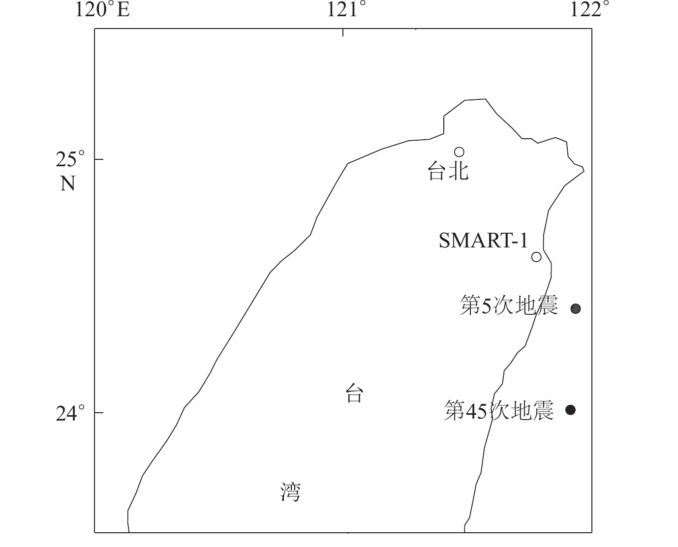
本文选取SMART-1台站的第5次和第45次地震记录的东西向(EW)和南北向(NS)水平加速度作为统计数据。第5次地震发生于1981年01月29日,震级为ML6.3,震中距30 km,震源深度25 km,截取的S波时间窗为6—11 s,数据采集间隔dt=0.01 s;第45次地震发生于1986年11月14日,震级为ML7.0,震中距79 km,震源深度7 km,截取的S波时间窗为9—29 s,数据采集间隔同样取dt=0.01 s。SMART-1台阵与两次地震的相对位置如图2所示。
![]() 图 2 两次地震震中位置示意图Figure 2. Schematic diagram of the epicenter location of two earthquakes
图 2 两次地震震中位置示意图Figure 2. Schematic diagram of the epicenter location of two earthquakes基于强震台阵观测资料对地震动空间变化的研究通常是以随机振动理论为基础,采用相干函数研究空间上任意两点地震动的统计相关性,其中最常用的是迟滞相干系数(常简称为相干系数),其表达式为
$$ \left|{\gamma }_{ jk} ( f{\text{,}}d ) \right|{\text{=}}\frac{\left|{\bar{S}}_{ jk} ( f ) \right|}{\sqrt{{\bar{S}}_{ j} ( f ) {\bar{S}}_{ k} ( f ) }} {\text{,}} $$ (1) 式中: f为频率;d为台站间距离;
$ {\bar S_{ j}} ( f ) $ ,$ {\bar S_{ k}} ( f ) $ 和$ {\bar S_{ jk}} ( f ) $ 分别为场点 j和k的两个时间过程的自功率谱$ {S_{ j}} ( f ) $ ,$ {S_{ k}} ( f ) $ 和互功率谱$ {S_{ jk}} ( f ) $ 的平滑谱,本文采用的平滑窗为11阶汉宁(Hamming)窗。根据相干函数的变化趋势,研究人员提出过很多相干函数模型(Loh,1985;Harichandran, Vanmanmarche,1986;Hao,1989;Abraham son et al,1991;屈铁军等,1996;刘先明等,2004;李英民等,2013),本文选用Loh模型(Loh,1985)对函数系数进行回归分析,该模型的数学表达式为
$$ \left| {\gamma ( f{\text{,}} d ) } \right| {\text{=}} \exp [ - ( a{\text{+}} b{f^2} ) d ] {\text{,}} $$ (2) 式中a和b为拟合系数。
2. 相干系数计算
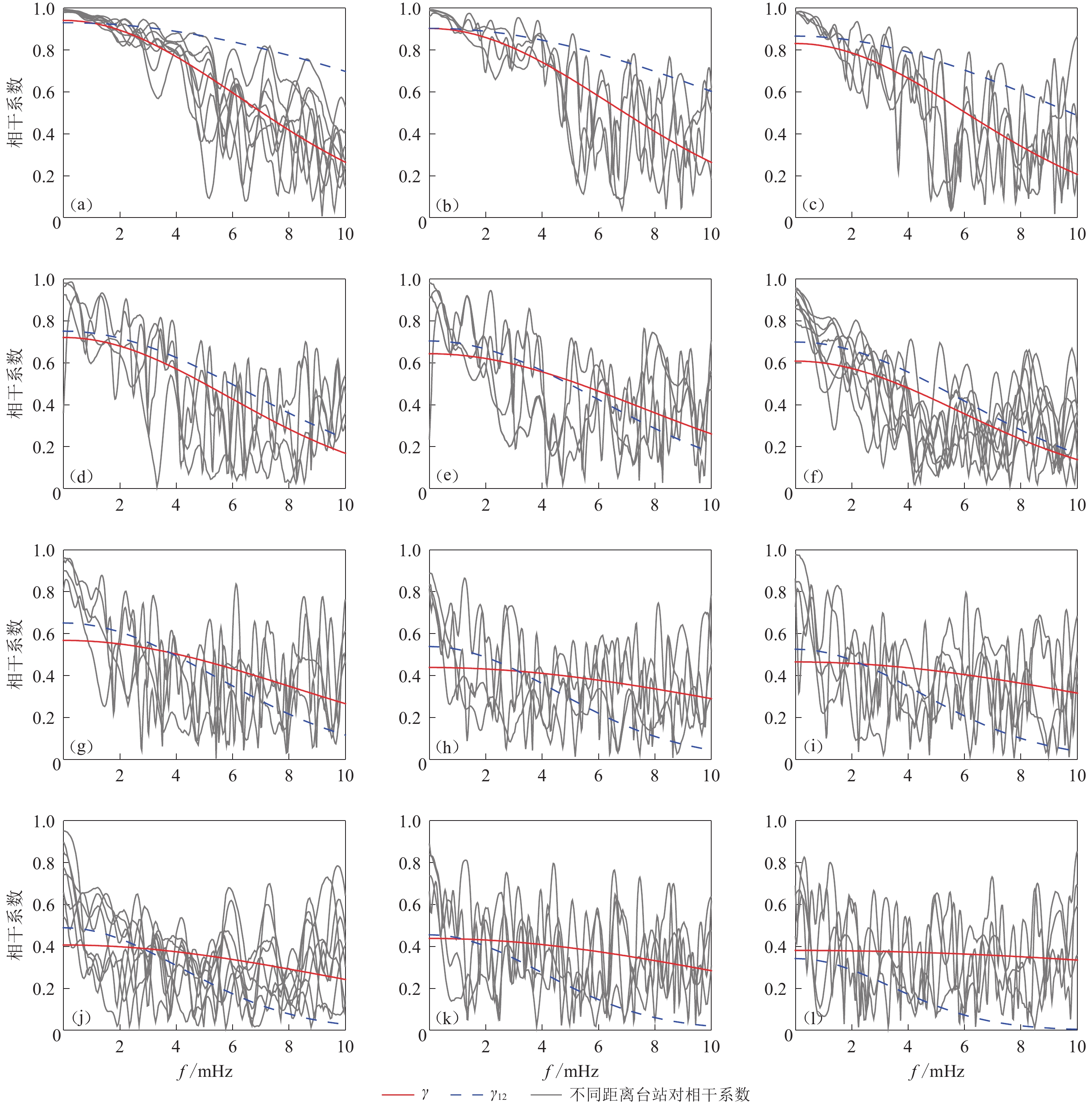
根据台站间的相对位置,本文组合了12种不同距离的台站对。不同的台站间距和对应的台站对数量列于表1。根据式(1)可以计算不同距离的台站对相干系数(包括EW和NS两个水平方向),如图3和图4中的实线所示。根据式(2)的相干函数模型,本文采用2种方法对相干函数进行拟合。一种是分别对不同台站间距d的相干函数拟合,得到的拟合参数a和b列于表2,对应的拟合相干函数曲线如图3和图4中以γ表示的红色实线。另一种是对所有12种不同台站间距d的相干函数进行拟合(图3,4蓝色虚线),得到的拟合参数 a和 b见表2中对应的12d。
表 1 台站间距和对应的台站对及数量Table 1. Distance between stations and the corresponding number of station pairs台站距离d/m 台站对 台站对个数 台站距离d/m 台站对 台站对个数 200 C00−I03 4 1 200 I06−M12 2 282 I03−I06 2 1 732 M06−O09 2 400 I03−I09 2 1 800 I03−O03 2 800 I03−M03 2 2 000 C00−O03 4 980 I03−M06 2 2 200 I03−O09 2 1 000 C00−M03 4 3 000 M03−O09 2 ![]() 图 3 不同间距的相干系数γ与根据所有不同间距的相干系数γ12的拟合曲线对比(以第5次地震为例)Figure 3. Comparison between fitting curves with lagged coherency γ of different distances and fitting curves with lagged coherency γ12 of all distance (taking the 5th earthquake as an example)(a) d=200 m;(b) d=282 m;(c) d=400 m;(d) d=800 m;(e) d=980 m;(f) d=1 000 m;(g) d=1 200 m; (h) d=1 732 m;(i) d=1 800 m;(j) d=2 000 m;(k) d=2 200 m;(l) d=3 000 m
图 3 不同间距的相干系数γ与根据所有不同间距的相干系数γ12的拟合曲线对比(以第5次地震为例)Figure 3. Comparison between fitting curves with lagged coherency γ of different distances and fitting curves with lagged coherency γ12 of all distance (taking the 5th earthquake as an example)(a) d=200 m;(b) d=282 m;(c) d=400 m;(d) d=800 m;(e) d=980 m;(f) d=1 000 m;(g) d=1 200 m; (h) d=1 732 m;(i) d=1 800 m;(j) d=2 000 m;(k) d=2 200 m;(l) d=3 000 m![]() 图 4 不同间距的相干系数γ与根据所有不同间距的相干系数γ12的拟合曲线对比 (以第45次地震为例)Figure 4. Comparison between fitting curve with lagged coherency γ of different distances and fitting curve with lagged coherency γ12 of all distance(taking the 45th earthquake as an example)(a) d=200 m;(b) d=282 m;(c) d=400 m;(d) d=800 m;(e) d=980 m;(f) d=1 000 m;(g) d=1 200 m; (h) d=1 732 m;(i) d=1 800 m;(j) d=2 000 m;(k) d=2 200 m;(l) d=3 000 m表 2 基于Loh相干函数模型的拟合系数结果Table 2. Fitting coefficient results based on Loh coherency function model
图 4 不同间距的相干系数γ与根据所有不同间距的相干系数γ12的拟合曲线对比 (以第45次地震为例)Figure 4. Comparison between fitting curve with lagged coherency γ of different distances and fitting curve with lagged coherency γ12 of all distance(taking the 45th earthquake as an example)(a) d=200 m;(b) d=282 m;(c) d=400 m;(d) d=800 m;(e) d=980 m;(f) d=1 000 m;(g) d=1 200 m; (h) d=1 732 m;(i) d=1 800 m;(j) d=2 000 m;(k) d=2 200 m;(l) d=3 000 m表 2 基于Loh相干函数模型的拟合系数结果Table 2. Fitting coefficient results based on Loh coherency function model台站距离d/m 第5次地震 第45次地震 a b a b 200 0.476 49 0.000 72 0.299 25 0.001 60 282 0.328 58 0.000 38 0.359 96 0.001 10 400 0.300 20 0.000 29 0.461 33 0.000 88 800 0.305 26 0.000 21 0.408 63 0.000 46 980 0.325 09 0.000 11 0.449 52 0.000 23 1 000 0.260 01 0.000 13 0.496 97 0.000 38 1 200 0.208 47 0.000 08 0.471 04 0.000 16 1 732 0.193 98 0.000 04 0.475 44 0.000 06 1 800 0.180 25 0.000 04 0.425 02 0.000 05 2 000 0.169 69 0.000 06 0.449 15 0.000 07 2 200 0.161 71 0.000 04 0.374 76 0.000 05 3 000 0.164 18 0.000 00 0.321 45 0.000 01 12d 0.189 77 0.000 08 0.357 08 0.000 36 由表2可知,不同台站间距d的相干函数拟合参数各不相同,并且与由12种不同台站间距d的所有相干函数拟合得到的参数也有很大差别。对比图3和图4中拟合曲线γ和γ12可以看出,两曲线完全不重合,且在台站间距d的统计范围内,当距离较大(如2200 m,3000 m)或距离较小(如200 m,282 m)时,相干系数的差别更明显。这是因为相干系数具有随间距增大而减小的趋势,当对所有12种不同台站间距d的相干系数进行拟合时,其结果相对更接近所有相干系数的平均值,也就更接近中间距离的相干系数。
3. 对拟合系数a和b的修正
3.1 系数a和b的修正函数模型的选取和修正结果
因不同台站距离的相干函数拟合系数不一致,导致对于相同的台站距离,由不同台站间距得到的相干系数拟合曲线与由所有不同台站间距得到的相干系数拟合曲线相比有误差,且对于某些距离误差较大(图3,4)。因此,在通常采用根据所有相干系数得到的拟合参数进行地震动场的人工合成时,就会出现短距离的模拟地震动相关性偏大,长距离的模拟地震动相关性偏小的现象。由图5可见:拟合系数a和b随台站距离d的分布不在一条直线上,且有一定的离散;而由所有不同台站间距得到的相干系数拟合结果并不随距离d发生变化,实际显示为一条直线,因此,由不同的拟合系数a和b得到的同一距离的相干系数存在差别的。为了减小因拟合系数的差异而造成拟合曲线γ与γ12的误差,本节将对不同距离相干系数的拟合系数a和b进行修正,即对a和b进行二次拟合。根据a和b的分布规律,比较了几组a和b的拟合函数形式(只与距离d有关),最终选用参数a和b的拟合函数表达式分别为
![]() 图 5 第5次(蓝色)和第45次(红色)地震的参数a (a),b (b)值随距离的变化及修正结果Figure 5. Changes of parameters a (a) and b (b) with distance and modified results of the 5th (blue) and the 45th (red) earthquakes
图 5 第5次(蓝色)和第45次(红色)地震的参数a (a),b (b)值随距离的变化及修正结果Figure 5. Changes of parameters a (a) and b (b) with distance and modified results of the 5th (blue) and the 45th (red) earthquakes$$ a {\text{=}} {a_1} {d^{{a_2}}} {\text{+}} {a_3} {\text{,}} $$ (3) $$ b{\text{=}}{b}_{1} ( d{{\text{+}}{b}_{2} ) }^{{b}_{3}}{\text{,}} $$ (4) 式中a1,a2,a3和b1,b2,b3分别为二次拟合系数,最终得到a和b的修正结果列于表3。
表 3 a和b二次拟合系数的修正结果Table 3. Modified results of a and b地震 a1 a2 a3 b1 b2 b3 第5次 0.733 53 −0.133 37 −0.482 98 0.000 10 −0.114 25 −0.805 45 第45次 −0.000 57 −3.410 92 0.432 46 0.000 82 0.573 00 −2.470 90 3.2 修正后的相干函数模型及结果
将修正后的系数a和b代入式(2),得到修正后的相干函数模型为
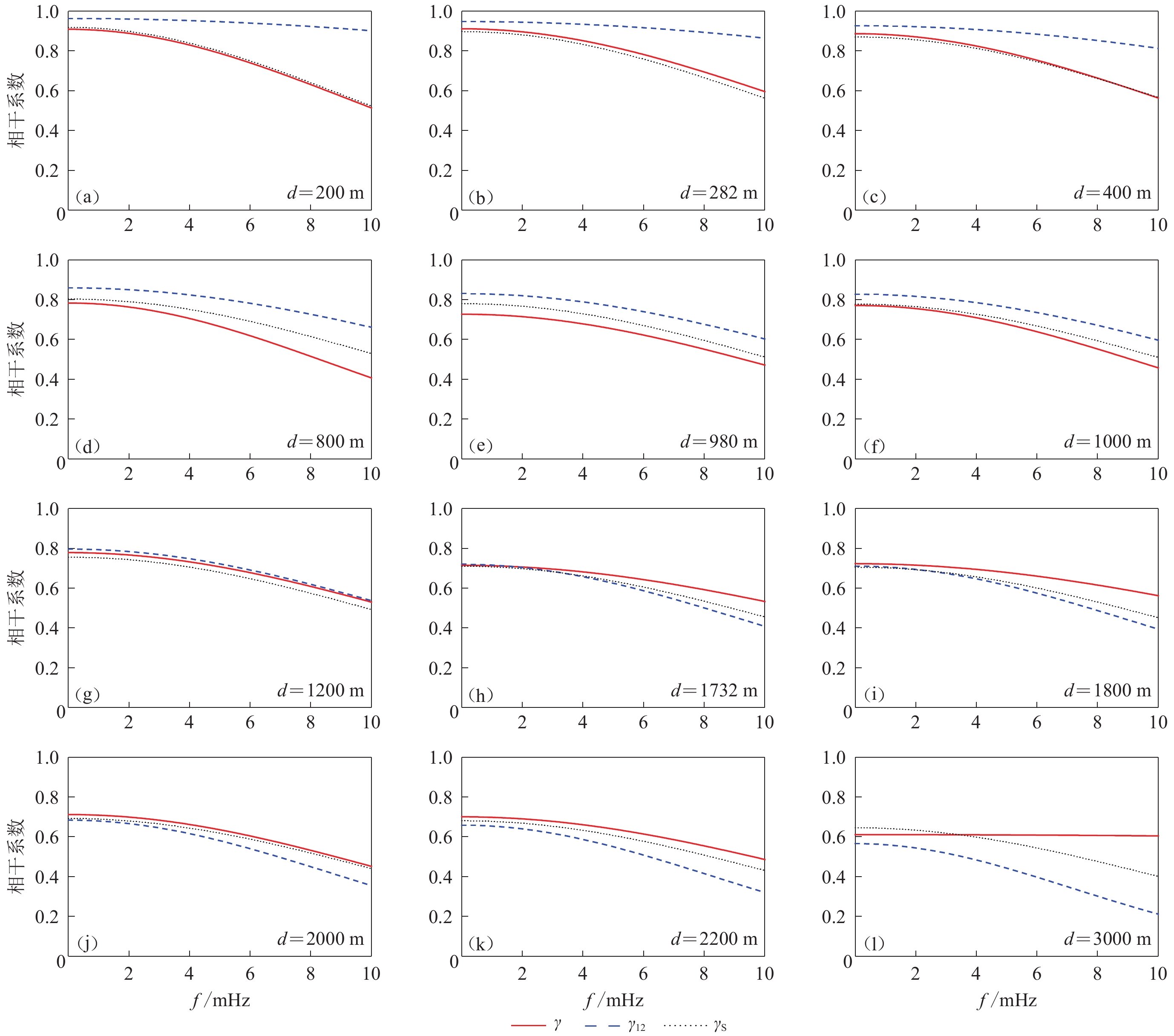
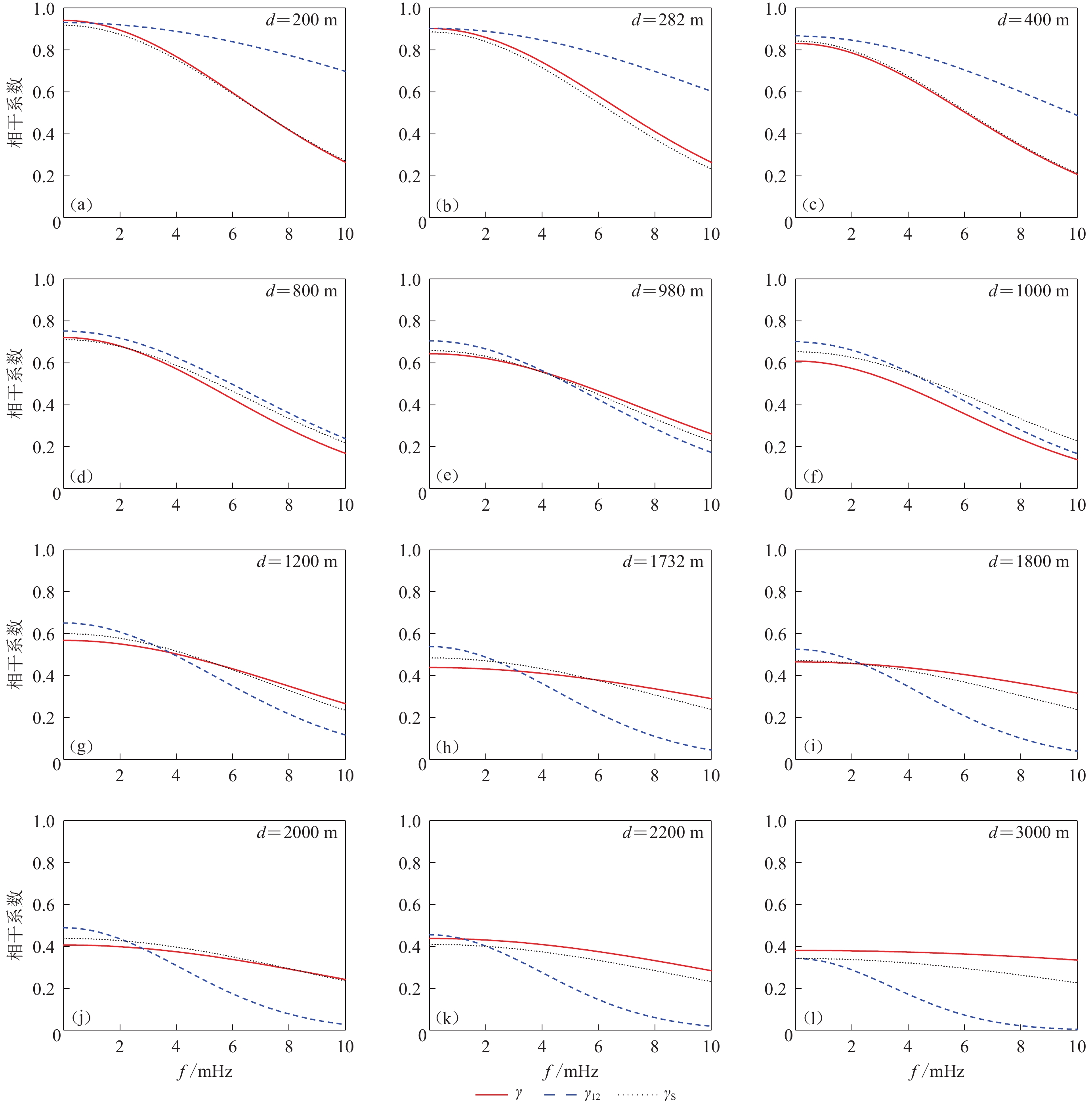
$$ \left|{\gamma }_{{\rm{s}}}(f{\text{,}} d)\right|{\text{=}}{{\rm{exp}}} { [ - ( {a}_{1} {d}^{{a}_{2}}+{a}_{3} ) {\text{+}}{b}_{1} ( d{{\text{+}}{b}_{2})}^{{b}_{3}}{f}^{2} ] d }{\text{,}} $$ (5) 式中系数a1,a2,a3和b1,b2,b3的值列于表3。将表3中修正后的拟合系数代入式(4),可计算得到修正后的相干系数γs,并与先前的两种拟合结果进行对比,结果如图6和图7所示。图中红色实线γ为各单独台站距离下相干系数的拟合结果,蓝色虚线γ12为所有12个台站距离的拟合结果,黑色虚线γs为修正后的相干系数拟合结果。从图中的比较可以看出,修正后的相干系数拟合结果γs与各单独台站距离下相干系数的拟合结果γ的符合程度得到了明显提高,保证了相干系数的拟合精度。
![]() 图 6 基于Loh相干函数模型,不同间距的相干系数γ、由所有不同间距的相干系数γ12和修正后的相干系数γs拟合曲线对比(以第5次地震为例)Figure 6. Based on Loh coherency function model,comparison of fitting curve with lagged coherency γ of different distances,fitting curve with lagged coherency γ12 of all distance and fitting curve with lagged coherency γs of modified parameter (taking the 5th earthquake as an example)
图 6 基于Loh相干函数模型,不同间距的相干系数γ、由所有不同间距的相干系数γ12和修正后的相干系数γs拟合曲线对比(以第5次地震为例)Figure 6. Based on Loh coherency function model,comparison of fitting curve with lagged coherency γ of different distances,fitting curve with lagged coherency γ12 of all distance and fitting curve with lagged coherency γs of modified parameter (taking the 5th earthquake as an example)![]() 图 7 基于LOH相干函数模型,不同间距的相干系数γ、根据所有不同间距的相干系数γ12和修正后的相干系数γs拟合曲线对比(以第45次地震为例)Figure 7. Based on Loh coherency function model,comparison of fitting curve of lagged coherency γ of different distances,fitting curve of lagged coherency of all distance γ12 and fitting curve with lagged coherency of modified parameter γs (taking the 45th earthquake as an example)
图 7 基于LOH相干函数模型,不同间距的相干系数γ、根据所有不同间距的相干系数γ12和修正后的相干系数γs拟合曲线对比(以第45次地震为例)Figure 7. Based on Loh coherency function model,comparison of fitting curve of lagged coherency γ of different distances,fitting curve of lagged coherency of all distance γ12 and fitting curve with lagged coherency of modified parameter γs (taking the 45th earthquake as an example)为了便于应用,对两次相干系数统一进行拟合,可得到由单独台站距离拟合的相干系数(红色实线γ)和由所有12个台站距离拟合的相干系数(蓝色虚线γ12),结果如图8所示。采用上述相同方法,对 a和 b进行修正,得到的统一修正结果列于表4,而相应的修正后的相干系数拟合结果如图8中黑色虚线γs所示。可以看出,修正后的结果得到了较为明显的改进。
![]() 图 8 不同间距的相干系数经修正前γ、后γs的拟合曲线与根据所有不同间距的相干系数γ12拟合曲线的比较(以两次地震为例)Figure 8. Comparison of fitting curve of lagged coherency γ of different distances,fitting curve of lagged coherency γ12 of all distance and fitting curve with lagged coherency γs of modified parameter (take two earthquakes as examples)表 4 a和 b的统一修正结果Table 4. Unified modified results of a and b
图 8 不同间距的相干系数经修正前γ、后γs的拟合曲线与根据所有不同间距的相干系数γ12拟合曲线的比较(以两次地震为例)Figure 8. Comparison of fitting curve of lagged coherency γ of different distances,fitting curve of lagged coherency γ12 of all distance and fitting curve with lagged coherency γs of modified parameter (take two earthquakes as examples)表 4 a和 b的统一修正结果Table 4. Unified modified results of a and ba1 a2 a3 b1 b2 b3 −0.022 1.759 9 0.416 3 0.011 9 1.531 3 −4.367 4. 讨论与结论
本文采用了SMART-1台阵两次地震的水平向分量加速度记录,计算分析了台站距离d对地震动空间相干函数的影响。首先计算了不同间距台站对的相干函数,然后选用Loh相干函数模型对不同距离的相干函数,以及所有不同距离的相干函数分别进行了参数拟合,再对由不同距离相干函数的拟合参数进行二次回归,比较了所有的拟合结果,得到结果如下:
1) 不同台站间距强震记录的相干函数拟合参数的离散性很大,但根据各个不同距离的拟合参数计算得到的相干函数符合随距离的增大而减小的规律。
2) 对于某一特定距离,由该距离的相干函数值得到的拟合结果γ与由所有不同距离相干函数值得到的拟合结果γ12存在明显的差异,距离越大或越小,偏差越大。这种偏差将会造成在采用由所有相干系数得到的拟合参数进行地震动场的人工合成时,短距离的模拟地震动相关性偏大,长距离的模拟地震动相关性偏小。
3) 对不同距离相干函数的拟合参数进行二次回归,对于相同的距离,根据修正后的参数得到的拟合相干函数γs与该距离单独得到的拟合相干函数γ符合程度得到了明显提高,这说明本文的修正结果更适合应用于实际的所有不同场点间距(200—3000 m)的空间地震动的人工模拟。
4) 给出了基于Loh相干函数模型的SMART-1台阵第5次和第45次地震的修正拟合参数,以及两次地震统一的修正拟合参数。
-
![]()
图 2 两次地震震中位置示意图
Figure 2. Schematic diagram of the epicenter location of two earthquakes
![]()
图 3 不同间距的相干系数γ与根据所有不同间距的相干系数γ12的拟合曲线对比(以第5次地震为例)
Figure 3. Comparison between fitting curves with lagged coherency γ of different distances and fitting curves with lagged coherency γ12 of all distance (taking the 5th earthquake as an example)
(a) d=200 m;(b) d=282 m;(c) d=400 m;(d) d=800 m;(e) d=980 m;(f) d=1 000 m;(g) d=1 200 m; (h) d=1 732 m;(i) d=1 800 m;(j) d=2 000 m;(k) d=2 200 m;(l) d=3 000 m
![]()
图 4 不同间距的相干系数γ与根据所有不同间距的相干系数γ12的拟合曲线对比 (以第45次地震为例)
Figure 4. Comparison between fitting curve with lagged coherency γ of different distances and fitting curve with lagged coherency γ12 of all distance(taking the 45th earthquake as an example)
(a) d=200 m;(b) d=282 m;(c) d=400 m;(d) d=800 m;(e) d=980 m;(f) d=1 000 m;(g) d=1 200 m; (h) d=1 732 m;(i) d=1 800 m;(j) d=2 000 m;(k) d=2 200 m;(l) d=3 000 m
![]()
图 5 第5次(蓝色)和第45次(红色)地震的参数a (a),b (b)值随距离的变化及修正结果
Figure 5. Changes of parameters a (a) and b (b) with distance and modified results of the 5th (blue) and the 45th (red) earthquakes
![]()
图 6 基于Loh相干函数模型,不同间距的相干系数γ、由所有不同间距的相干系数γ12和修正后的相干系数γs拟合曲线对比(以第5次地震为例)
Figure 6. Based on Loh coherency function model,comparison of fitting curve with lagged coherency γ of different distances,fitting curve with lagged coherency γ12 of all distance and fitting curve with lagged coherency γs of modified parameter (taking the 5th earthquake as an example)
![]()
图 7 基于LOH相干函数模型,不同间距的相干系数γ、根据所有不同间距的相干系数γ12和修正后的相干系数γs拟合曲线对比(以第45次地震为例)
Figure 7. Based on Loh coherency function model,comparison of fitting curve of lagged coherency γ of different distances,fitting curve of lagged coherency of all distance γ12 and fitting curve with lagged coherency of modified parameter γs (taking the 45th earthquake as an example)
![]()
图 8 不同间距的相干系数经修正前γ、后γs的拟合曲线与根据所有不同间距的相干系数γ12拟合曲线的比较(以两次地震为例)
Figure 8. Comparison of fitting curve of lagged coherency γ of different distances,fitting curve of lagged coherency γ12 of all distance and fitting curve with lagged coherency γs of modified parameter (take two earthquakes as examples)
表 1 台站间距和对应的台站对及数量
Table 1 Distance between stations and the corresponding number of station pairs
台站距离d/m 台站对 台站对个数 台站距离d/m 台站对 台站对个数 200 C00−I03 4 1 200 I06−M12 2 282 I03−I06 2 1 732 M06−O09 2 400 I03−I09 2 1 800 I03−O03 2 800 I03−M03 2 2 000 C00−O03 4 980 I03−M06 2 2 200 I03−O09 2 1 000 C00−M03 4 3 000 M03−O09 2  下载: 导出CSV
表 2 基于Loh相干函数模型的拟合系数结果
Table 2 Fitting coefficient results based on Loh coherency function model
台站距离d/m 第5次地震 第45次地震 a b a b 200 0.476 49 0.000 72 0.299 25 0.001 60 282 0.328 58 0.000 38 0.359 96 0.001 10 400 0.300 20 0.000 29 0.461 33 0.000 88 800 0.305 26 0.000 21 0.408 63 0.000 46 980 0.325 09 0.000 11 0.449 52 0.000 23 1 000 0.260 01 0.000 13 0.496 97 0.000 38 1 200 0.208 47 0.000 08 0.471 04 0.000 16 1 732 0.193 98 0.000 04 0.475 44 0.000 06 1 800 0.180 25 0.000 04 0.425 02 0.000 05 2 000 0.169 69 0.000 06 0.449 15 0.000 07 2 200 0.161 71 0.000 04 0.374 76 0.000 05 3 000 0.164 18 0.000 00 0.321 45 0.000 01 12d 0.189 77 0.000 08 0.357 08 0.000 36
下载: 导出CSV
表 3 a和b二次拟合系数的修正结果
Table 3 Modified results of a and b
地震 a1 a2 a3 b1 b2 b3 第5次 0.733 53 −0.133 37 −0.482 98 0.000 10 −0.114 25 −0.805 45 第45次 −0.000 57 −3.410 92 0.432 46 0.000 82 0.573 00 −2.470 90
下载: 导出CSV
表 4 a和 b的统一修正结果
Table 4 Unified modified results of a and b
a1 a2 a3 b1 b2 b3 −0.022 1.759 9 0.416 3 0.011 9 1.531 3 −4.367
下载: 导出CSV
-
丁海平,罗翼,饶威波,朱越. 2018. 截止频率的取值对地震动空间相干函数统计结果的影响[J]. 地震学报,40(5):664–672. Ding H P,Luo Y,Rao W B,Zhu Y. 2018. The influence of cut-off frequency on the statistical results of spatial coherency function of seismic ground motion[J]. Acta Seismologica Sinica,40(5):664–672 (in Chinese).
李英民,吴哲骞,陈辉国. 2013. 地震动的空间变化特性分析与修正相干模型[J]. 振动与冲击,32(2):164–170. doi: 10.3969/j.issn.1000-3835.2013.02.032 Li Y M,Wu Z Q,Chen H G. 2013. Analysis and modeling for characteristics of spatially varying ground motion[J]. Journal of Vibration and Shock,32(2):164–170 (in Chinese).
刘先明,叶继红,李爱群. 2004. 竖向地震动场的空间相干函数模型[J]. 工程力学,21(2):140–144. doi: 10.3969/j.issn.1000-4750.2004.02.024 Liu X M,Ye J H,Li A Q. 2004. Space coherency function model of vertical ground motion[J]. Engineering Mechanics,21(2):140–144 (in Chinese).
屈铁军,王君杰,王前信. 1996. 空间变化的地震动功率谱的实用模型[J]. 地震学报,18(1):55–62. Qu T J,Wang J J,Wang Q X. 1996. A practical model for the power spectrum of spatial variant ground motion[J]. Acta Seismologica Sinica,18(1):69–79.
饶威波,丁海平,罗翼. 2018. 台站间距d 的分布对地震动空间相干函数的影响[J]. 地震工程与工程振动,38(3):103–109. Rao W B,Ding H P,Luo Y. 2018. The influence of the distribution of station distance d on the ground motion’s coherence function[J]. Earthquake Engineering and Engineering Dynamics,38(3):103–109 (in Chinese).
Abrahamson N A,Bolt B A,Darragh R B,Penzien J,Tsai Y B. 1987. The SMART-I accelerograph array (1980−1987):A review[J]. Earthq Spectra,3(2):263–287. doi: 10.1193/1.1585428
Abrahamson N A,Schneider J F,Stepp J C. 1991. Empirical spatial coherency functions for application to soil-structure interaction analyses[J]. Earthq Spectra,7(1):1–27. doi: 10.1193/1.1585610
Abrahamson N A. 1993. Spatial variation of multiple support inputs[C]//Proceedings of the 1st U.S. Seminar on Seismic Evaluation and Retrofit of Steel Bridges. San Francisco, California: A Caltrans and University of California at Berkeley Seminar.
Bi K M,Hao H,Chouw N. 2013. 3D FEM analysis of pounding response of bridge structures at a canyon site to spatially varying ground motions[J]. Adv Struct Eng,16(4):619–640. doi: 10.1260/1369-4332.16.4.619
Chopra A K,Wang J T. 2010. Earthquake response of arch dams to spatially varying ground motion[J]. Earthq Eng Struct Dyn,39(8):887–906.
der Kiureghian A. 1996. A coherency model for spatially varying ground motions[J]. Earthq Eng Struct Dyn,25(1):99–111. doi: 10.1002/(SICI)1096-9845(199601)25:1<99::AID-EQE540>3.0.CO;2-C
Hao H. 1989. Effects of Spatial Variation of Ground Motions on Large Multiply-Supported Structures[R]. Berkeley: University of California: 18–27.
Harichandran R S,Vanmarcke E H. 1986. Stochastic variation of earthquake ground motion in space and time[J]. J Eng Mech,112(2):154–174. doi: 10.1061/(ASCE)0733-9399(1986)112:2(154)
Li C,Hao H,Li H N,Bi K M,Chen B K. 2017. Modeling and simulation of spatially correlated ground motions at multiple onshore and offshore sites[J]. J Earthq Eng,21(3):359–383. doi: 10.1080/13632469.2016.1172375
Liu C,Gao R. 2018. Design method for steel restrainer bars on railway bridges subjected to spatially varying earthquakes[J]. Eng Struct,159:198–212. doi: 10.1016/j.engstruct.2018.01.001
Loh C H. 1985. Analysis of the spatial variation of seismic waves and ground movements from SMART-1 array data[J]. Earthq Eng Struct Dyn,13(5):561–581. doi: 10.1002/eqe.4290130502
Park D,Sagong M,Kwak D Y,Jeong C G. 2009. Simulation of tunnel response under spatially varying ground motion[J]. Soil Dyn Earthq Eng,29(11/12):1417–1424.
Wu Y X,Gao Y F,Zhang N,Li D Y. 2016. Simulation of spatially varying ground motions in V-shaped symmetric canyons[J]. J Earthq Eng,20(6):992–1010. doi: 10.1080/13632469.2015.1010049
Zerva A. 2009. Spatial Variation of Seismic Ground Motions: Modeling and Engineering Applications[M]. New York: CRC Press: 96–119.
-
期刊类型引用(0)
其他类型引用(1)


计量
- 文章访问数: 246
- HTML全文浏览量: 119
- PDF下载量: 42
- 被引次数: 1
