

qP wave ray tracing in FMM elastic TTI media based on phase velocity prediction
-
摘要:
快速准确地计算走时和射线路径是实现地震成像和反演的关键。在各向异性介质中,地震波的传播速度会随传播方向的变化而变化,这使得求解各向异性条件程函方程时,相速度的精确估计和计算变得非常复杂和困难,进而影响各向异性介质中走时和射线路径的计算精度和效率。为此,提出了一种基于相速度预测的射线追踪方法,该方法根据波的传播规律以及斯奈尔方程,推导出一种相速度预测公式,解决了各向异性条件程函方程中相速度求解困难的问题,实现了快速稳定的射线追踪。数值算例表明,本文所提出的改进算法明显提高了走时计算精度,耗时也仅比各向同性快速推进增加了14%,在复杂模型的应用中也表现出较强的适应性和稳定性。
Abstract:Fast and accurate calculation of travel time and ray path of seismic waves are two key problems in the field of seismic imaging and inversion. Solving these two problems plays a key role in the in-depth study of the fine structure of the Earth’s interior, the efficient exploration of the distribution of different types of resources underground, and even the scientific prediction of possible natural disasters. However, the situation becomes more complex when anisotropic media are involved. In such media, the velocity of seismic waves does not remain constant as in isotropic media, but varies with the propagation direction of seismic waves. This characteristic makes it a challenging task to calculate the propagation time of seismic waves and to determine the ray paths in anisotropic media. The conventional isotropic fast marching method (FMM) shows excellent performance advantages in solving the travel time problem in isotropic media. It is able to produce results relatively quickly and accurately due to its efficient algorithm and stable computational process. However, when we try to apply the method to solve the Eikonal equation under anisotropic conditions, we are faced with a critical aspect: the need for an accurate estimation of the phase velocity. This is because in an anisotropic medium, the velocity, anisotropy parameter and stratigraphic dip are not constant, and their dynamic changes make the calculation of the propagation direction complicated. The complex calculation of the propagation direction further increases the difficulty of phase velocity estimation. As a key parameter describing the velocity of seismic waves in a given direction, the accuracy of the phase velocity estimation is like the first domino in the chain, which directly affects the subsequent propagation time and the final accuracy of the ray path calculation. Any small deviation in the phase velocity estimate can be amplified in the subsequent calculations, leading to a large deviation of the final results from the actual situation.
In this paper, the fast marching method (FMM) for anisotropic media, which is a mature and widely used method, is taken as a solid basis for an in-depth study. Through rigorous theoretical derivation and practical verification, a phase velocity estimation method for tilted transversely isotropic (TTI) media and an anisotropic ray tracing method based on the principle of phase velocity prediction (PVP) are proposed. The method cleverly inherits the outstanding features of speed and stability of isotropic FMM, while maintaining the same level of computational accuracy as isotropic FMM, ensuring reliability and accuracy of results. A phase velocity prediction formula for TTI media has been derived. The formula can directly and accurately calculate the corresponding changes in phase velocity based on the changes in key factors such as seismic wave velocity, anisotropy parameter and stratigraphic dip. It greatly simplifies the complicated process of solving the anisotropic Eikonal equation and breaks the bottleneck of the previous methods in terms of computational efficiency and accuracy. It also greatly improves the computational efficiency of ray tracing, making the calculation process more efficient and faster, and at the same time significantly improves the computational accuracy, providing a more reliable and accurate basis for subsequent processing and interpretation of seismic exploration data.
In order to comprehensively and thoroughly verify the computational efficiency and accuracy of the method in practical applications, simulation experiments are carried out on a number of representative typical models. First, a unified theoretical model is used as the first test object. The model is relatively simple in structure and has a clear theoretical analytical solution, which can provide a clear reference standard for the accuracy verification of the method. Through comparative analyses, the results clearly show that the computational results obtained by the method are in high agreement with the theoretical results, which strongly verifies the excellent performance of the method in terms of accuracy. Then, the vertical transverse isotropy (VTI) reference model and Marmousi model are further tested. The results show that this method has small calculation error and good stability, and can be applied to ray tracing of complex structures. In addition, in order to further quantify the performance of the method, a multi-source near-surface numerical simulation test is also carried out. A model of complex near-surface structure is designed, and the wave fields of multiple sources are simulated by finite difference method. The seismic record of the model is simulated and its first arrival time is picked up. Then, ray tracing and travel time calculation are carried out by using this method, and the results are compared with those of finite difference simulation. The calculation errors and time of isotropic FMM and anisotropic PVP-FMM are statistically analyzed. The results show that both of them have the same calculation error, and the average error is very small. The error of anisotropic PAP-FMM is 43% less than that of anisotropic FMM without phase velocity prediction. A computer with 2.4 GHz CPU is used for ray tracing. The total time consumption of 913 source for isotropic FMM and PAP-FMM are 326 seconds and 372 seconds respectively. Because anisotropic FMM increases the calculation links of phase velocity and group velocity, the time consumption is increased by 10% compared with isotropic FMM. PVP-FMM added a phase angle prediction link, which increased the time consumption by 14%. In summary, this method has the same computational efficiency as isotropic FMM, and also has good adaptability and stability for near-surface models.
-
Keywords:
- anisotropy /
- fast marching method /
- ray tracing /
- phase velocity
-
引 言
在地震波处理和成像中,快速且准确的射线追踪和走时计算是至关重要的,尤其在走时层析成像(Klibanov et al,2023)、微震源定位(Grechka et al,2015)和地震叠前偏移(Garabito,2021)等应用中起着关键作用。随着技术的不断发展,基于各向同性介质假设的技术已经不能完全满足实际生产应用的需要。各向异性介质射线追踪方法由各向同性方法发展而来,分为两大类:一是传统的两点间射线追踪方法(Julian,Gubbins,1977),该类方法可达到很高的计算精度,但对于复杂介质可能存在阴影区或走时局部最小问题(王东鹤等,2016);二是基于网格的射线追踪方法,主要包括最短路径法和有限差分解程函方程法。最短路径法具有良好的稳健性,但为保证计算精度,需要较细的网格,致使其计算成本较高(Nakanishi,Yamaguchi,1986;Zhou,Greenhalgh,2005;张美根等,2006;赵爱华等,2006;赵后越,张美根,2014;邴琦等,2020)。相比之下,有限差分求解程函方程法可有效弥补传统射线追踪法的不足,在不增加网格密度的情况下提供高效且较为精确的数值(周洪波,张关泉,1994;赵烽帆等,2014)。
快速扫描法(fast sweeping method,缩写为FSM)和快速推进法(fast marching method,缩写为FMM)是有限差分求解程函方程最常用的两种算法。FSM利用局部解程函方程来更新格点走时信息,通过反复扫描模型以稳定走时场,通常采用上风插值方案求局部解(Zhao,2004)。因此,FSM被广泛用于求解各向异性介质的qP波走时问题(Waheed et al,2015;Hao et al,2018;Tro et al,2023)。然而,FSM在复杂模型中需要更多的迭代次数以获得高精度的走时,较为耗时。Sethian (1999)提出的FMM则采用上风差分格式来求解局部程函方程,利用窄带延拓来重建走时波前,并使用堆排序技术保存走时信息,以加速寻找最小走时。这一方法显著提高了计算效率,将计算量从波前扩展法的O(N3)减小到O(NlgN)。由于各向异性群速度确定的能量传播方向与相速度给出的波前传播方向不同,原始的FMM只适用于各向同性介质,不能可靠地用于求解各向异性方程。为解决这一问题,Sethian和Vladimirsky (2003)提出了一种适用于各向异性介质的有序迎风方法。随后,许多学者提出了改进的FMM方法,以适用于各向异性介质,并开展了进一步的研究,使其得以快速发展。
Lelièvre等(2011)将FMM方法扩展到非结构三维四面体网格中进行初至地震走时计算。Treister和Haber (2016)提出了一种适用于因式分解程函方程的FMM算法,有效地解决了由震源奇异性引起的不精确数值解问题。Waheed和Alkhalifah (2017)利用因式分解方法研究了倾斜横向各向同性(tilted transverse isotropy,缩写为TTI)方程问题,通过迭代求解一个因式分解的倾斜椭圆各向异性程函方程序列,能够更好地描述各向异性波前。Sun等(2017)提出了一种联合3D的走时计算方法,在震源附近小范围内使用计算精度较高的波前构建法计算走时,在剩余区域使用FMM算法计算走时,改善了震源附近区域计算精度不高的问题。Le Bouteiller等(2019)在间断伽辽金方法(discontinuous Galerkin method,缩写为DGM)中引入FSM算法来求解三维程函方程,降低了计算的复杂度。Waheed (2020)将TTI介质程函方程表示为椭圆各向同性方程序列后利用FMM可快速准确地计算TTI介质的走时,但计算工作量随着迭代次数的增加而增大,与各向同性FMM相比,算法实现变得更加复杂。因此,如何在求解各向异性程函方程时均衡计算效率和精准度是目前走时计算的一个挑战性问题。
针对上述问题,本文基于各向同性FMM思想提出一种基于相速度预测的各向异性FMM射线追踪方法(phase velocity prediction fast marching method,缩写为PVP-FMM)。首先,预测网格节点的相速度,再使用FMM计算网格节点波前时间;其次,计算每个网格的波前梯度,重构相速度矢量场;进一步,由相速度矢量场重构群速度矢量场;最后,由群速度矢量场插值计算射线路径和走时。该方法继承了各向异性FMM无条件稳定的特点,具有与各向同性FMM相同的计算效率和精度,能够适用于复杂构造的TTI介质射线追踪,具有良好的稳定性和较高的计算效率。
1. 各向异性程函方程建立
1.1 TTI介质程函方程
各向异性介质在高频近似条件下的程函方程可表示为(Vidale,1988)
$$ v_{\mathrm{P}}^2 ( \theta ) \nabla \tau · \nabla \tau=1\text{,} $$ (1) 式中,$\nabla $为梯度算子,τ为走时场计算中的当前走时,vP为各向异性介质准qP波的相速度。相速度与波前法向方向有关,Thomsen (1986)在弱各向异性条件下获得相速度的近似表达式为
$$ {v_{\mathrm{P}}} ( \theta ) ={v_{\mathrm{n}}} ( 1 + \varepsilon {\sin ^4}\theta + \delta {\sin ^2}\theta {\cos ^2}\theta ) \text{,} $$ (2) 式中,θ为相角,vn为地层法向方向速度,ε和δ都为汤姆森(Thomsen)参数。
Waheed (2020)将Alkhalifah (2000)提出的TTI介质程函方程分解成一系列椭圆方程,使用椭圆波前迭代拟合各向异性波前,但随着迭代次数增加的同时,也增加了计算成本。为此,本文直接利用式(1)求解各向异性波前,将其改写为
$$ {\left( {\frac{{ {\text{∂}} \tau }}{{ {\text{∂}} x}}} \right)^2} + {\left( {\frac{{ {\text{∂}} \tau }}{{ {\text{∂}} {\textit{z}} }}} \right)^2}=\frac{1}{{v_{\mathrm{n}}^2{{ ( 1 + \varepsilon {{\sin }^4}\theta + \delta {{\sin }^2}\theta {{\cos }^2}\theta ) }^2}}}=f ( \theta ) . $$ (3) 从式(3)中可以看出,如果能够知道其相速度,就可计算出相应的走时。与各向同性程函方程求解方法一样,只需在每个网格点计算二次多项式,不用在每个网格点上求解复杂的高阶多项式,与各向同性时具有相同的计算效率。因此相速度精确预测是使用式(3)求解各向异性波前的关键环节。
1.2 FMM方法离散化处理程函方程
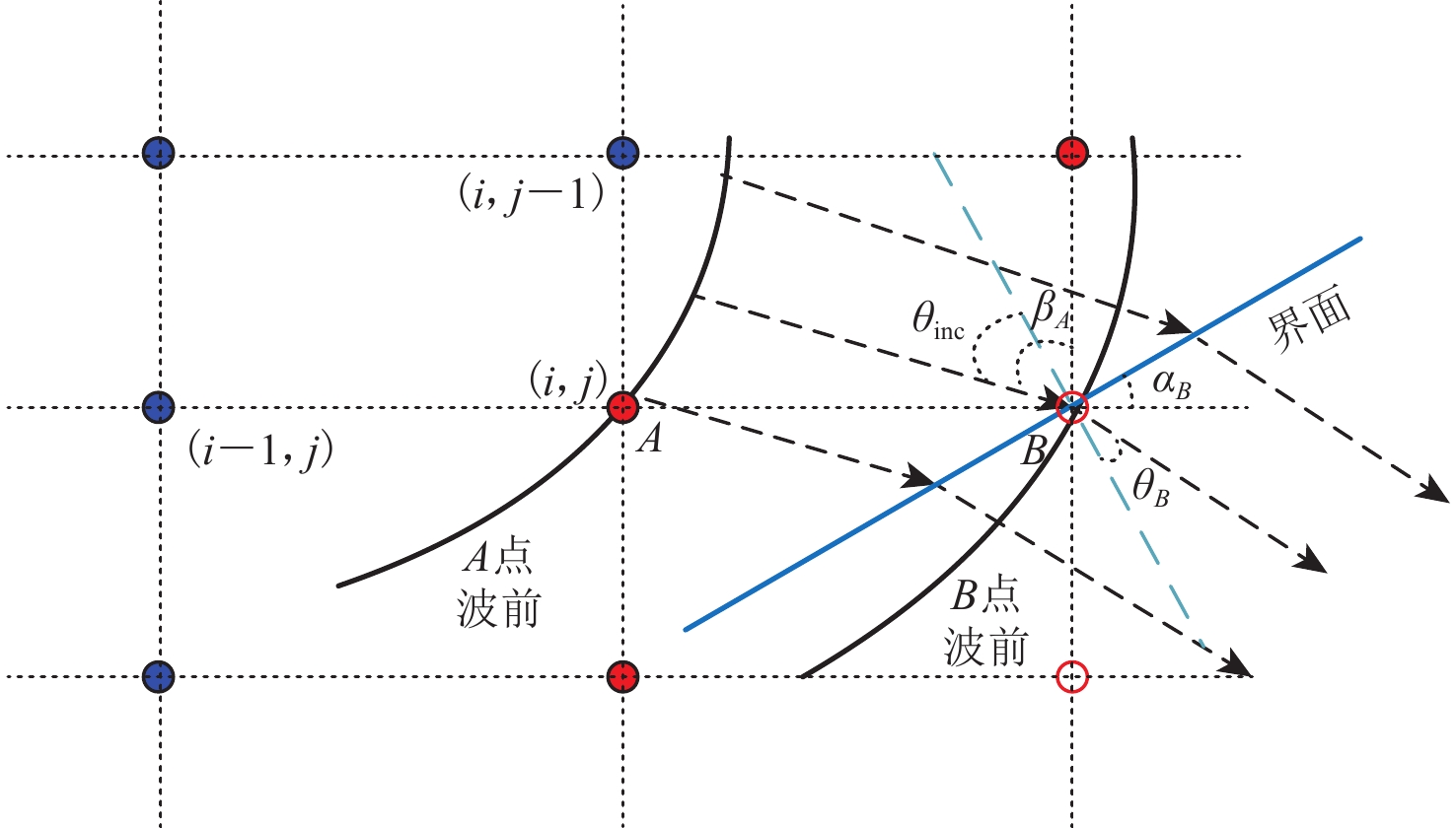
FMM算法将整个计算域划分为三个区域:上风区、波前区和下风区。波从上风区经过波前区传播至下风区,如图1所示。上风区为已经求解出走时的已知区域,波前区是正在求解的区域,下风区是还未求解的未知区域。在波前区的窄带内,寻找最小波前时间点,将其属性改为已知点的同时继续向下风区扩展,直至所有网格点都在上风区。
![]() 图 1 快速推进法(FMM)实现原理图Figure 1. Implementation schematic diagram of fast marching method (FMM)
图 1 快速推进法(FMM)实现原理图Figure 1. Implementation schematic diagram of fast marching method (FMM)在图1中,设节点A是波前区最小波前时间节点,节点B是其邻近的走时未知节点。由于点A的波前时间已知,可以计算波前梯度求出点A的波传播方向。当波由点A传播至点B时,如果两个节点的速度不同,传播方向会发生变化,从而使得节点B的传播方向和相角也是未知的。因此,在节点B使用式(3)求解波前时间的关键就是要预测相速度。
使用FMM方法对式(3)进行二阶上风差分格式离散。对于网格点(i, j),离散如下:
$$ \begin{gathered} { [ \max ( D_{i \text{,} j}^{ - x}\tau \text{,} - D_{i \text{,} j}^{ + x}\tau \text{,} 0 ) ] ^2} + { [ \max ( D_{i \text{,} j}^{ - {\textit{z}} }\tau \text{,} - D_{i \text{,} j}^{ + {\textit{z}} }\tau \text{,} 0 ) ] ^2}=f ( {\theta _{i \text{,} j}} ) \text{,} \\ f ( {\theta _{i \text{,} j}} ) =\frac{1}{{v_{i \text{,} j}^2{{ ( 1 + {\varepsilon _{i \text{,} j}}{{\sin }^4}{\theta _{i \text{,} j}} + {\delta _{i \text{,} j}}{{\sin }^2}{\theta _{i \text{,} j}}{{\cos }^2}{\theta _{i \text{,} j}} ) }^2}}} \text{,} \\ \end{gathered} $$ (4) 式中,$v_{i \text{,} j} $,${\varepsilon _{i \text{,} j}} $,${\delta _{i \text{,} j}} $,${\theta _{i \text{,} j}} $分别为地层法向速度、汤姆森参数和相角在节点(i, j)的值,$D_{i \text{,} j}^{ - x} $和$D_{i \text{,} j}^{ + x} $是待求点波前时间τ在x方向上的二阶差分运算符,表示为
$$ \begin{gathered} D_{i \text{,} j}^{ - x}\tau=\frac{{3{\tau _{i \text{,} j}} - 4{\tau _{i - 1 \text{,} j}} + {\tau _{i - 2 \text{,} j}}}}{{2\Delta x}} \text{,} D_{i \text{,} j}^{ + x}\tau=- \frac{{3{\tau _{i \text{,} j}} - 4{\tau _{i + 1 \text{,} j}} + {\tau _{i + 2 \text{,} j}}}}{{2\Delta x}} \text{,} \end{gathered} $$ (5) 式中Δx是x方向上的网格间距。z方向的前、后二阶差分计算与x方向前后二阶差分计算类似。这种迎风差分方案可确保信息从较低的波前时间值传播到较高的值。
2. 基于相速度预测的FMM波前重构
在地震波传播过程中,当地层参数变化时,其传播方向与相速度也会发生变化。当求解待求点B的波前时间时,如果依然采用已知点A的相速度进行计算,则波前时间就会存在一定误差。若这种误差累积扩散到整个计算域,则导致波前时间解的精度降低。为解决此问题,本文利用斯奈尔(Snell)方程推导出待求点与已知点间的相速度关系,进而得出相速度预测公式;再结合相速度预测公式与FMM算法求解波前时间;最后,采用群速度矢量场插值计算射线路径。
2.1 TTI介质相速度预测
如图2所示,假设地层参数在节点B处存在一个倾斜分界面。对于TTI介质,分界面两边的vn,ε和δ不同,根据斯奈尔定律,在分界面满足如下关系(邓怀群等,2000):
$$ \begin{split} p=\frac{{\sin {\theta _{{\rm{inc}}}}}}{{{v_{\rm{P}}} ( {\theta _{{\mathrm{inc}}}} ) }}=\frac{{\sin {\theta _{B}}}}{{{v_{\rm{P}}} ( {\theta _{B}} ) }} \text{,} \end{split} $$ (6) 式中,p为射线参数,θinc和θB分别为入射角和出射角,${{v_{\mathrm{P}}} ( {\theta _{{\mathrm{inc}}}} ) } $和${{v_{\mathrm{P}}} ( {\theta _{{B}}} ) } $分别为节点A和B处的相速度。式中出射角θB可表示为θB=θinc+Δθ,令x=sinθinc,式(6)可等价表示为
$$ p=\frac{x}{{{v_{\mathrm{n}}} ( 1 + \varepsilon {x^4} - \delta {x^4}+ \delta {x^2} ) }}. $$ (7) 为了便于计算,先对式(7)进行处理,令$f ( x ) =1 + \varepsilon {x^4} - \delta {x^4} + \delta {x^2}$,可知
$$ p{v_{\mathrm{n}}}f ( x ) =x\text{,} $$ (8) 对式(8)两边进行微分可得
$$ pf ( x ) {\mathrm{d}}{v_{\mathrm{n}}} + p{v_{\mathrm{n}}}{x^4}{\mathrm{d}}\varepsilon + ( {x^2} - {x^4} ) {\mathrm{d}}\delta \cdot p{v_{\mathrm{n}}} + p{v_{\mathrm{n}}} ( 4{x^3}\varepsilon - 4{x^3}\delta + 2x\delta ) {\mathrm{d}}x={\mathrm{d}}x. $$ (9) 根据式(8)可知,$p{v_{\mathrm{n}}}={x}/{{f ( x ) }} \text{,} pf ( x ) ={x}/{{{v_{\mathrm{n}}}}}$,将其代入式(9)有
$$ x\frac{{{\mathrm{d}}{v_{\mathrm{n}}}}}{{{v_{\mathrm{n}}}}} + \frac{x}{{f ( x ) }}{x^4}{\mathrm{d}}\varepsilon + \frac{x}{{f ( x ) }}{x^2} ( 1 - {x^2} ) {\mathrm{d}}\delta=\left\{ {1 - \frac{x}{{f ( x ) }} [ {4{x^3} ( \varepsilon - \delta ) + 2x\delta } ] } \right\}{\mathrm{d}}x\text{,} $$ (10) 进一步化简后可得
$$ \frac{\mathrm{d}x}{x}=\frac{f ( x ) }{1+3 ( \delta-\varepsilon ) x^4-x^2\delta}\frac{\mathrm{d}v_{\mathrm{n}}}{v_{\mathrm{n}}}+\frac{x^4}{1+3 ( \delta-\varepsilon ) x^4-x^2\delta}\mathrm{d}\varepsilon+\frac{x^2 ( 1-x^2 ) }{1+3 ( \delta-\varepsilon ) x^4-x^2\delta}\mathrm{d}\delta. $$ (11) 根据式(6)可知,待求点B的相速度为
$$ v_{\mathrm{P}} ( \theta_{\mathrm{B}} ) =v_{\mathrm{P}} ( \theta_{\mathrm{inc}} ) \frac{\sin ( \theta_{\mathrm{inc}}+\Delta\theta ) }{\sin\theta_{\mathrm{inc}}}=v_{\mathrm{P}} ( \theta_{\mathrm{inc}} ) \left(1+\frac{\Delta x}{x}\right)\text{,} $$ (12) 在求解过程中需满足$0 {\text{≤}} \sin ( {\theta_{{\mathrm{inc}}}} + \Delta \theta ) =x + \Delta x {\text{≤}} 1$的条件。将式(11)代入式(12)有
$$ v_{\mathrm{P}} ( \theta_{\mathrm{B}} ) =v_{\mathrm{P}} ( \theta_{\mathrm{inc}} ) \left[\frac{f ( x ) }{1+3 ( \delta-\varepsilon ) x^4-x^2\delta}\frac{\mathrm{d}v_{\mathrm{n}}}{v_{\mathrm{n}}}+\frac{x^4}{1+3 ( \delta-\varepsilon ) x^4-x^2\delta}\mathrm{d}\varepsilon+\frac{x^2 ( 1-x^2 ) }{1+3 ( \delta-\varepsilon ) x^4-x^2\delta}\mathrm{d}\delta\right]\text{,} $$ (13) 其中入射角θinc满足
$$ \theta_{\mathrm{inc}}=\beta_{\mathrm{\mathit{A}}}-\alpha_{\mathrm{\mathit{B}}}\text{,} $$ (14) 式中αB为节点B处的界面倾角,βA为节点A的传播方向与z轴的夹角。由于节点A的波前时间已是最小走时,不再变化,利用x方向与z方向上的∂τ/∂x与∂τ/∂z,传播方向βA表示为
$$ \mathrm{arctan}\beta_{\mathrm{\mathit{A}}}=\frac{\text{∂}\tau}{\text{∂}x}\mathord{\left/\vphantom{\frac{\text{∂}\tau}{\text{∂}x}\frac{\text{∂}\tau}{\text{∂}\text{z}}}\right.}\frac{\text{∂}\tau}{\text{∂}\text{z}}. $$ (15) 将式(14)和式(15)代入式(13),可得到待求点B的相速度vP(θB)。
对于待求点B的相角θB,利用式(4)以及式(13),求得待求点B的走时,再利用式(15)得到其传播方向βB,通过${\theta _{{B}}}={\beta _{{B}}} - {\alpha _{{B}}}$获得点B的相角。
因此,PVP-FMM方法求解波前时间最终分为三个步骤:首先,由点A的波前梯度计算点A的传播方向,再利用式(14)计算入射角;其次,根据相速度预测公式,计算出点B的相速度和相角;最后,将相速度代入式(4)中,计算出该点的波前时间,然后进行下一点预估,依此类推,直至所有网格点完成计算。
2.2 群速度矢量场和射线路径计算
各向异性射线追踪方法可分为四个步骤:首先,使用基于相速度预测的各向异性FMM方法计算网格节点波前时间;其次,计算每个网格的波前梯度,重构相速度矢量场;进一步,由相速度矢量场重构群速度矢量场;最后,由群速度矢量场插值计算射线路径和走时。具体计算步骤如下:① 利用式(4)和式(13)进行各向异性PVP-FMM波前时间计算,得到所有网格点波前时间场;② 在波前时间场中利用梯度运算可确定其整个相速度场,即
$$ \nabla\tau=\frac{\text{∂}\tau}{\text{∂}x}\boldsymbol{x}+\frac{\text{∂}\tau}{\text{∂}\text{z}}\boldsymbol{z},\boldsymbol{v}_{\mathrm{P}}=v_{\mathrm{P}}\frac{\nabla\tau}{\left|\nabla\tau\right|}\text{,} $$ (16) 式中,$\left| {\nabla \tau } \right|=1/{v_{\mathrm{P}}}(\theta )$,${{\nabla \tau }}/{{\left| {\nabla \tau } \right|}}={\boldsymbol{n}}\cos \theta + {\boldsymbol{t}} \sin \theta $,${\boldsymbol{ n}}$和$ {\boldsymbol{t}}$表示地层切向和法向的单位矢量;③ 通过群速度与相速度的关系可得到群速度场(Thomsen,1986),即
$$ {{\boldsymbol{v}}} _{\mathrm{g}}={{{\boldsymbol{v}}} _{\mathrm{P}}} ( \theta ) + \frac{{{\mathrm{d}}{v_{\mathrm{P}}}}}{{{\mathrm{d}}\theta }} ( {\boldsymbol{t}} \cos \theta- {\boldsymbol{n}} \sin \theta ) \text{,} $$ (17) 式中vg和vP(θ)分别表示群速度和相速度。对于TTI介质,相角由波前梯度方向经过坐标旋转变换后求得。${\boldsymbol{ t}}$可用相角以及${\boldsymbol{n}}$表示,即${\boldsymbol{t}}={1}/{{\sin \theta }}\left({{\nabla \tau }}/{{\left| {\nabla \tau } \right|}} - {\boldsymbol{n}} \cos \theta \right)$,因此式(17)中的群速度矢量也可表示为
$$ \begin{split} \boldsymbol{v}_{\mathrm{g}}= & \boldsymbol{v}_{\mathrm{P}} ( \theta ) +\frac{\mathrm{d}v_{\mathrm{P}}}{\mathrm{d}\theta} ( \boldsymbol{t}\cos\theta-\boldsymbol{n}\sin\theta ) =v_{\mathrm{P}}\frac{\nabla\tau}{\left|\nabla\tau\right|}+\frac{\mathrm{d}v_{\mathrm{P}}}{\mathrm{d}\theta} ( \boldsymbol{t}\cos\theta-\boldsymbol{n}\sin\theta ) =v_{\mathrm{P}}^2 ( \theta ) \nabla\tau+ \\ &\frac{\mathrm{d}v_{\mathrm{P}}}{\mathrm{d}\theta}\left(\frac{\cos\theta}{\sin\theta}\frac{\nabla\tau}{\left|\nabla\tau\right|}-\boldsymbol{n}\frac{\cos^2\theta}{\sin\theta}-\boldsymbol{n}\sin\theta\right)=v_{\mathrm{P}}^2 ( \theta ) \nabla\tau+\frac{\mathrm{d}v_{\mathrm{P}}}{\mathrm{d}\theta}\left(\frac{\nabla\tau}{|\nabla\tau|}\cos\theta-\boldsymbol{n}\right)\frac{1}{\sin\theta} \text{,} \end{split} $$ (18) 式中$ {\boldsymbol{n}}= {{\boldsymbol{z}}} \cos \alpha + {\boldsymbol{x}}\sin \alpha $;④ 射线路径由接收点开始,逆着群速度矢量场方向可以一直追踪到源点,其方向由邻近节点的群速度方向插值求出。走时由每个网格的射线长度除以群速度后求和获得。
3. 数值算例
基于均匀速度TTI模型、速度倾斜渐变的TTI模型、垂直横向各向同性(vertical transverse isotropy,缩写为VTI )模型、Marmousi模型以及近地表模型计算了五种模型的走时和射线路径,以此计算结果分析本文所提的方法在计算效率和计算精度上的性能。
3.1 均匀速度TTI模型
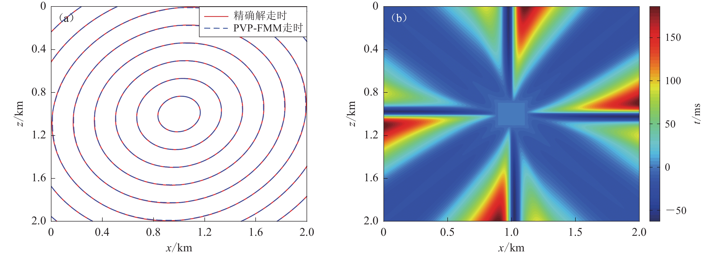
为了测试本文方法的准确性,设计一个均匀TTI模型进行试算。速度为2 km/s,模型横向、纵向尺寸均为0—2 km,网格间距均为10 m,倾角θ=45°,各向异性参数ε=0.1,δ=0.1,震源位于模型中央(1 km,1 km)。图3是均匀模型走时及其绝对误差的对比结果,其中:图3a为PVP-FMM计算的走时与精确解的对比,可以看出使用本文方法计算得到的走时与精确解基本吻合;图3b为走时绝对误差,从中可以看出,本文方法的最大走时误差约为1.5 ms,初步验证了本文方法的正确性。
![]() 图 3 均匀模型走时及误差对比(a) 走时对比;(b) 走时绝对误差对比Figure 3. Comparison of travel time and its error for homogeneous model(a) Comparison of travel time;(b) Comparison of absolute error of travel time
图 3 均匀模型走时及误差对比(a) 走时对比;(b) 走时绝对误差对比Figure 3. Comparison of travel time and its error for homogeneous model(a) Comparison of travel time;(b) Comparison of absolute error of travel time3.2 速度倾斜渐变的TTI模型
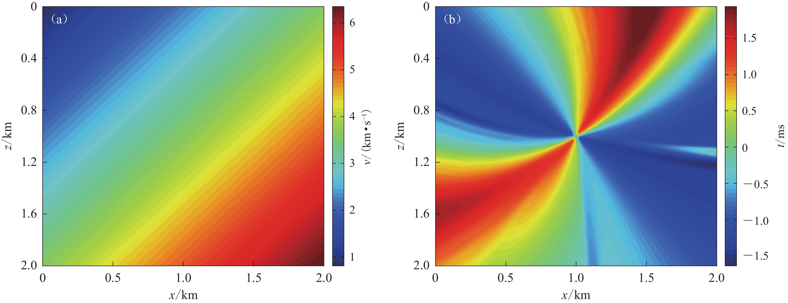
为了测试本文方法在TTI模型上的性能,设计了一个地层法向速度倾斜渐变的TTI模型。模型纵横向尺寸均为2 km,网格间距均为10 m,各向异性参数ε=0.16,δ=0.04,θ=45°。如图4a所示,其模型速度随深度的增加而增大,初始速度为800 m/s,深度每增加1 m速度增加2 m/s。图4b为PVP-FMM与无相角预测方法计算的波前时间之差。其中,无相角预测方法直接利用波前已知的与邻近节点相速度近似的FMM,将其缩写为No-PVP-FMM。
![]() 图 4 TTI模型走时之差对比(a) 速度模型;(b) PVP-FMM与No-PVP-FMM走时之差Figure 4. Comparison of travel time difference for TTI model(a) Velocity model;(b) Travel time difference between PVP-FMM and No-PVP-FMM
图 4 TTI模型走时之差对比(a) 速度模型;(b) PVP-FMM与No-PVP-FMM走时之差Figure 4. Comparison of travel time difference for TTI model(a) Velocity model;(b) Travel time difference between PVP-FMM and No-PVP-FMM从图4b走时绝对误差图可以看出,在其水平位置(45°方向)的误差基本为零,这是因为相角为零时,传播误差与ε和δ无关,误差最小,但是水平位置(45°方向)到90°方向误差逐渐增大,是由相角变化所致,90°到地层法向方向的误差则是由速度变化差异较大所引起。
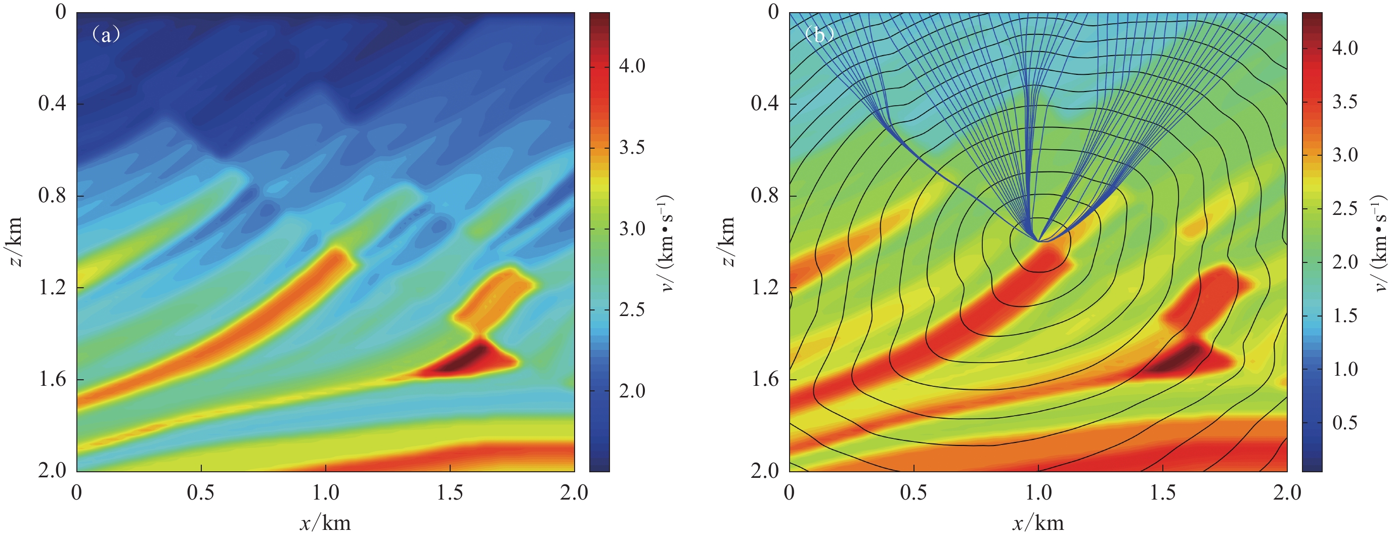
图5为炮点位于TTI模型中心时,利用本文方法计算所得的射线追踪过程。首先利用PVP-FMM方法计算得到所有网格点的波前时间场(图5a);其次,利用式(16)得到其相速度矢量场(图5b);然后根据式(18)获得群速度矢量场(图5c);最后,射线路径由接收点开始,逆着群速度矢量场方向一直追踪到炮点,如图5d所示。由图5可知,射线、等时线的密度都与模型参数的变化相符合。
![]() 图 5 利用本文方法PVP-FMM计算所得的射线追踪过程(炮点位于模型中心)(a) 波前时间场;(b) 相速度矢量场;(c) 群速度矢量场;(d) 射线路径Figure 5. The ray tracing process calculated by PVP-FMM in this paper (the shot point is located in the center of the model)(a) Wave front time field;(b) Phase velocity vector field;(c) Group velocity vector field; (d) Ray path
图 5 利用本文方法PVP-FMM计算所得的射线追踪过程(炮点位于模型中心)(a) 波前时间场;(b) 相速度矢量场;(c) 群速度矢量场;(d) 射线路径Figure 5. The ray tracing process calculated by PVP-FMM in this paper (the shot point is located in the center of the model)(a) Wave front time field;(b) Phase velocity vector field;(c) Group velocity vector field; (d) Ray path3.3 VTI模型
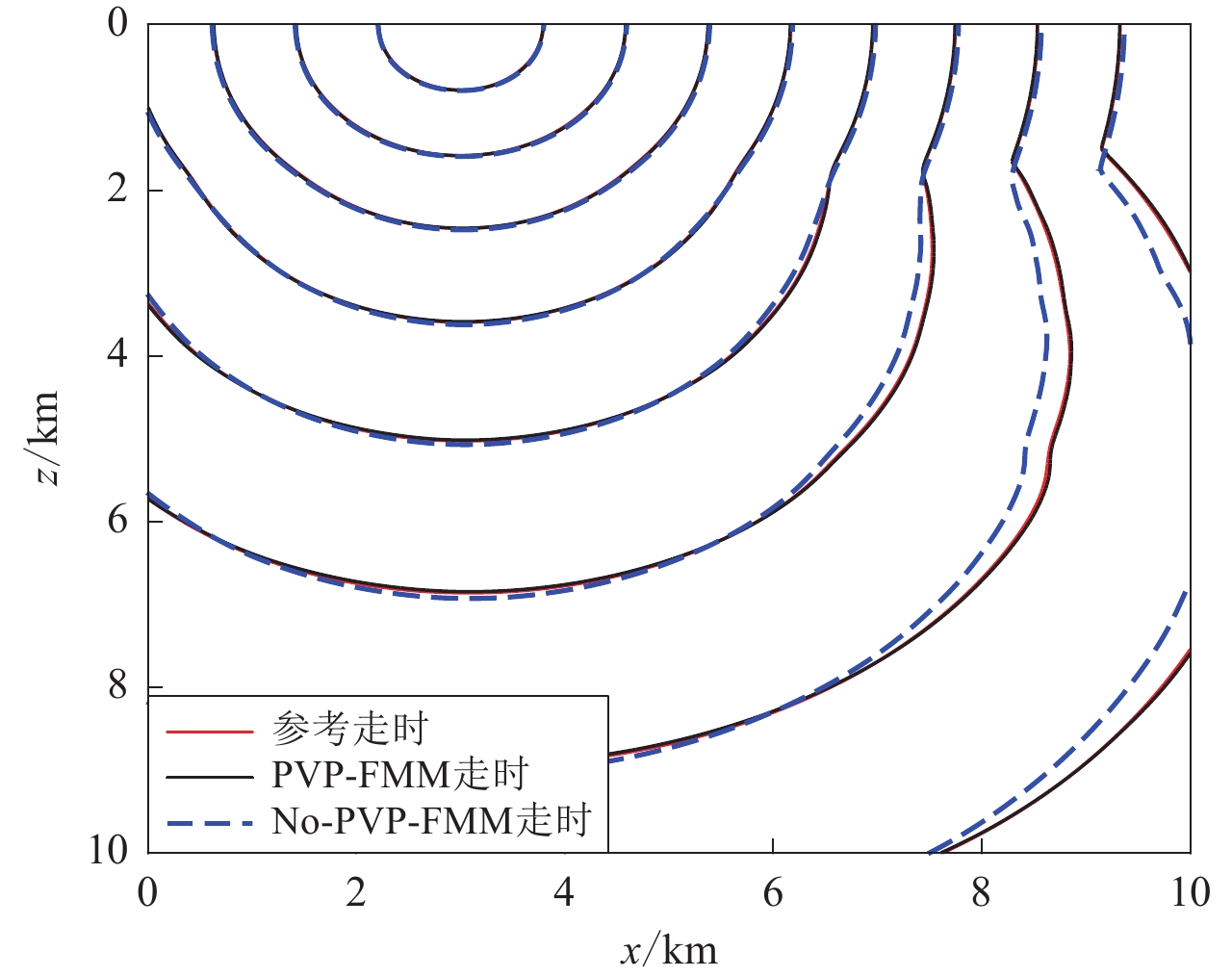
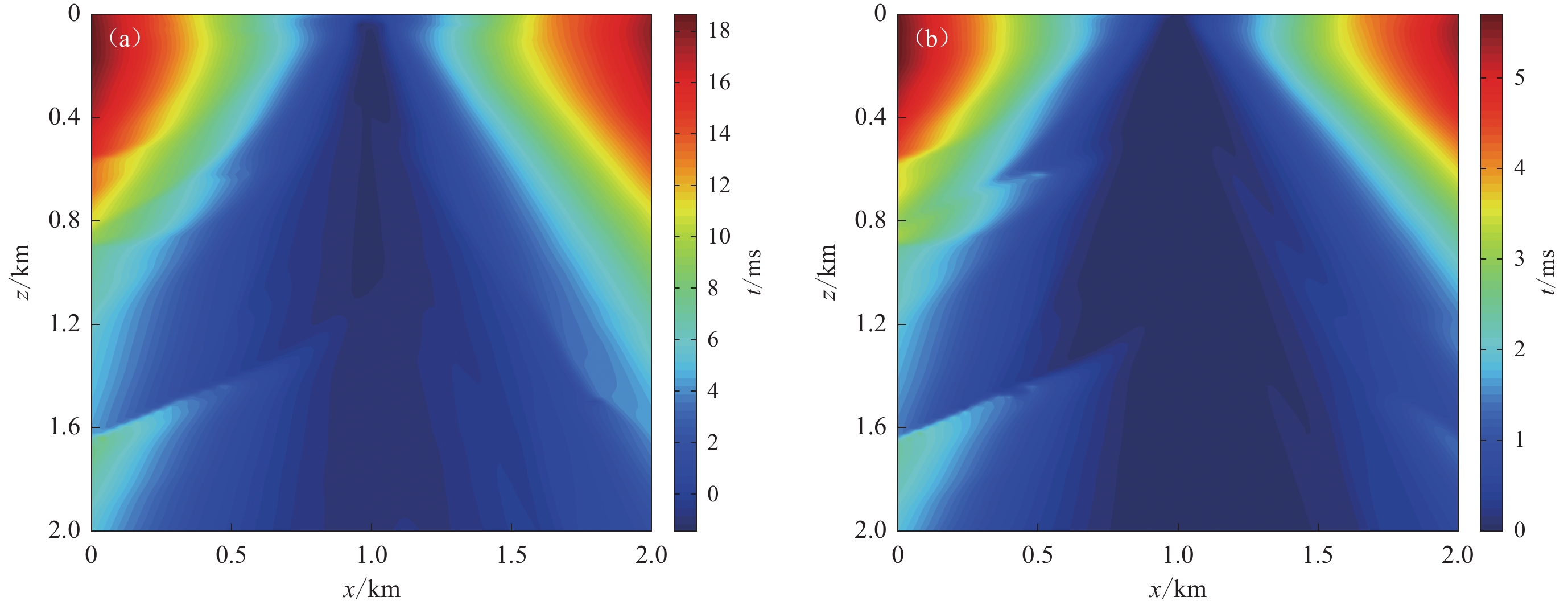
SEG Advanced modeling (SEAM)盐丘模型有多个数据集,这里我们采用其模型的一部分来验证本文方法的效果。模型参数为:模型横向、纵向坐标范围均为0—10 km,将其划分为201×201的网格,网格间距为50 m,各向异性介质参数ε=0.2,δ=0.12,模型的炮点位置在(3 km,0)处,模型速度如图6a所示。对该模型分别使用PVP-FMM和No-PVP-FMM方法进行走时计算和射线追踪,图6b为PVP-FMM的结果,图7为两种方法的结果与参考值的对比。图7中红色为SEAM公司所公布的参考走时解(Fehler,Keliher,2011),黑色为PVP-FMM方法,蓝色为No-PVP-FMM方法,从图中可以看出,两种算法之间差异明显,尤其在速度变化较大的地方本文方法与参考解吻合得很好,而No-PVP-FMM方法却在一些地方偏差较大。在走时误差图(图8)中也可以看出,No-PVP-FMM方法计算的解析解与参考解的最大误差约为0.14 s,本文方法计算结果与参考解的最大误差为0.018 s,可以发现本文方法比No-PVP-FMM方法的误差更小,得到的走时更加精确。
![]() 图 6 VTI模型追踪结果(a) 速度模型;(b) 波前等时线及射线追踪Figure 6. Ray tracing results of VTI model(a) Velocity model;(b) Wavefront isochron and ray path
图 6 VTI模型追踪结果(a) 速度模型;(b) 波前等时线及射线追踪Figure 6. Ray tracing results of VTI model(a) Velocity model;(b) Wavefront isochron and ray path3.4 Marmousi模型
为了验证本文方法处理复杂模型的性能,对Marmousi模型进行了测试。该模型大小为2 km×2 km,网格为101×101,网格间距为20 m,ε=0.16,δ=0.04,速度如图9a所示。图9b是源点位于模型中央时本文方法的计算结果。
![]() 图 8 走时绝对误差图Figure 8. Comparison of absolute error of travel time(a) No-PVP-FMM;(b) PVP-FMM
图 8 走时绝对误差图Figure 8. Comparison of absolute error of travel time(a) No-PVP-FMM;(b) PVP-FMM![]() 图 9 Marmousi模型追踪结果(a) 速度模型;(b) 波前等时线及射线追踪Figure 9. Ray tracing results of Marmousi model(a) Velocity model;(b) Wavefront isochron and ray path
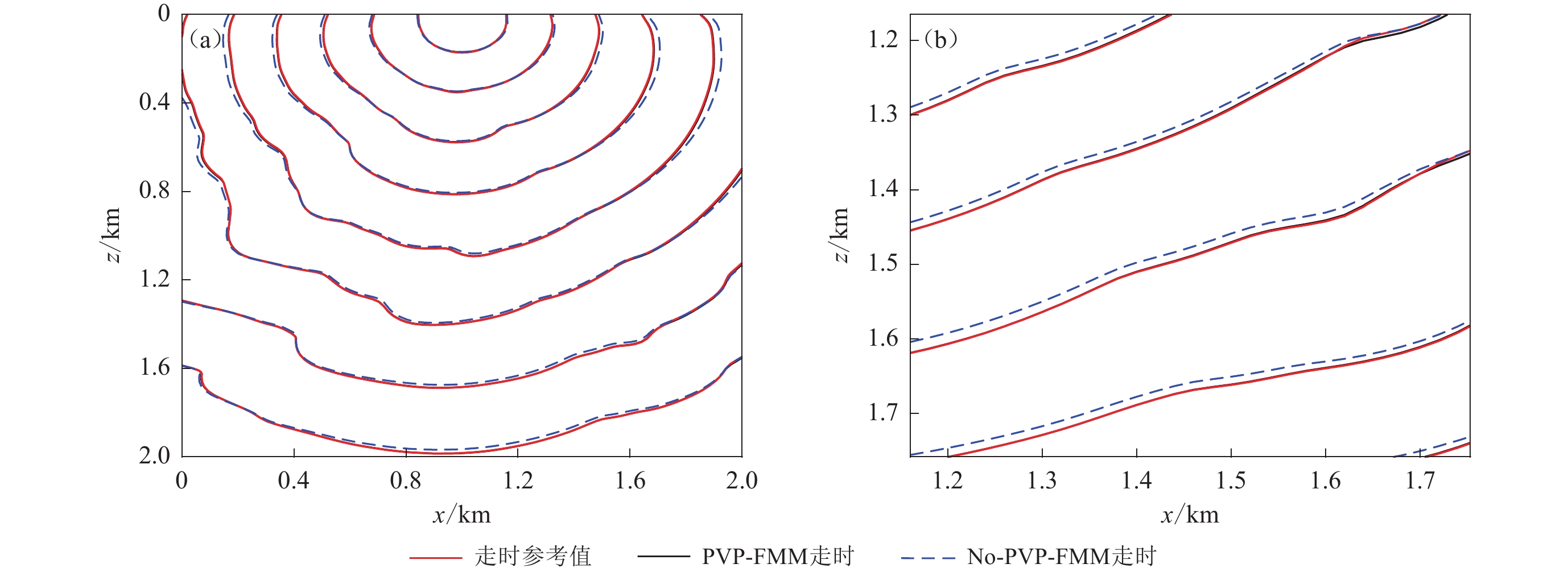
图 9 Marmousi模型追踪结果(a) 速度模型;(b) 波前等时线及射线追踪Figure 9. Ray tracing results of Marmousi model(a) Velocity model;(b) Wavefront isochron and ray path将震源位置移动到地面(1 km,0)后,分别使用PVP-FMM和No-PVP-FMM方法对模型进行计算。图10显示了两种方法获得的等时线与参考解之间的对比及误差图。图10a为全局图,图10b为局部放大图。从全局图中可知,两种方法的等时线结果几乎重合,但在速度变化快的地方可以看出明显的差异;在图10b的局部放大图中也可看出,No-PVP-FMM在发生速度变化大的区域内出现较大的偏差。走时绝对误差如图11所示,从图中可以看出,PVP-FMM算法明显比No-PVP-FMM的误差更小,可以说明PVP-FMM方法能明显改善速度变化剧烈区域的计算精度,针对复杂模型有更好的计算精度。
![]() 图 10 走时等值线对比图(a) 走时对比;(b) 局部放大图Figure 10. Comparison map of travel time contour(a) Comparison of travel time;(b) Local enlarged image
图 10 走时等值线对比图(a) 走时对比;(b) 局部放大图Figure 10. Comparison map of travel time contour(a) Comparison of travel time;(b) Local enlarged image![]() 图 11 走时绝对误差图Figure 11. Comparison of absolute error of travel time(a) No-PVP-FMM;(b) PVP-FMM
图 11 走时绝对误差图Figure 11. Comparison of absolute error of travel time(a) No-PVP-FMM;(b) PVP-FMM3.5 近地表数值模拟
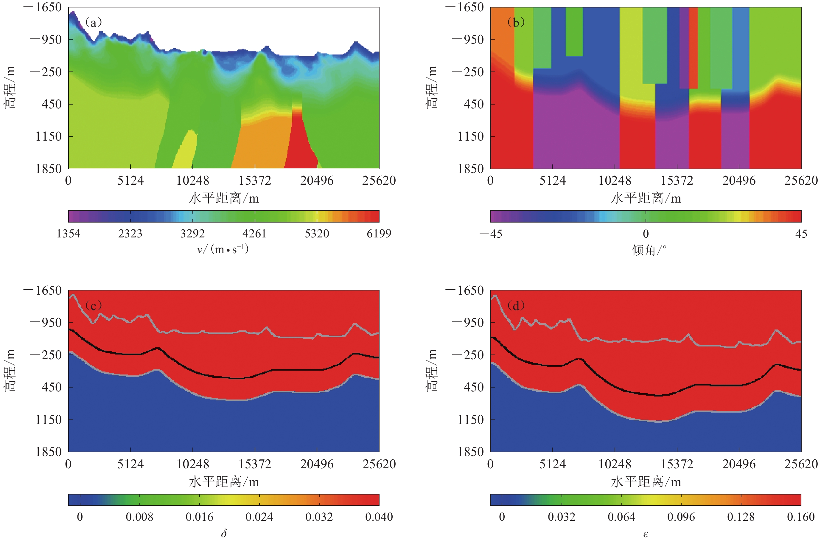
最后,为了测试本文算法在近地表各向异性模型中的实用性,根据实际地表状况,本文设计了一个地表起伏、地下结构复杂的近地表TTI模型。速度模型和地层倾角模型如图12a和12b所示,近地表各向异性参数值为ε=0.16,δ=0.04,随着深度的变化,参数也随之变化,如图12c和12d所示,观测系统设计了913个震源,每个震源有215个接收点。
![]() 图 12 近地表模型(a) 速度模型;(b) 倾角模型;(c) δ模型;(d) ε模型Figure 12. Near-surface models(a) Velocity;(b) Dip model;(c) δ model;(d) ε model
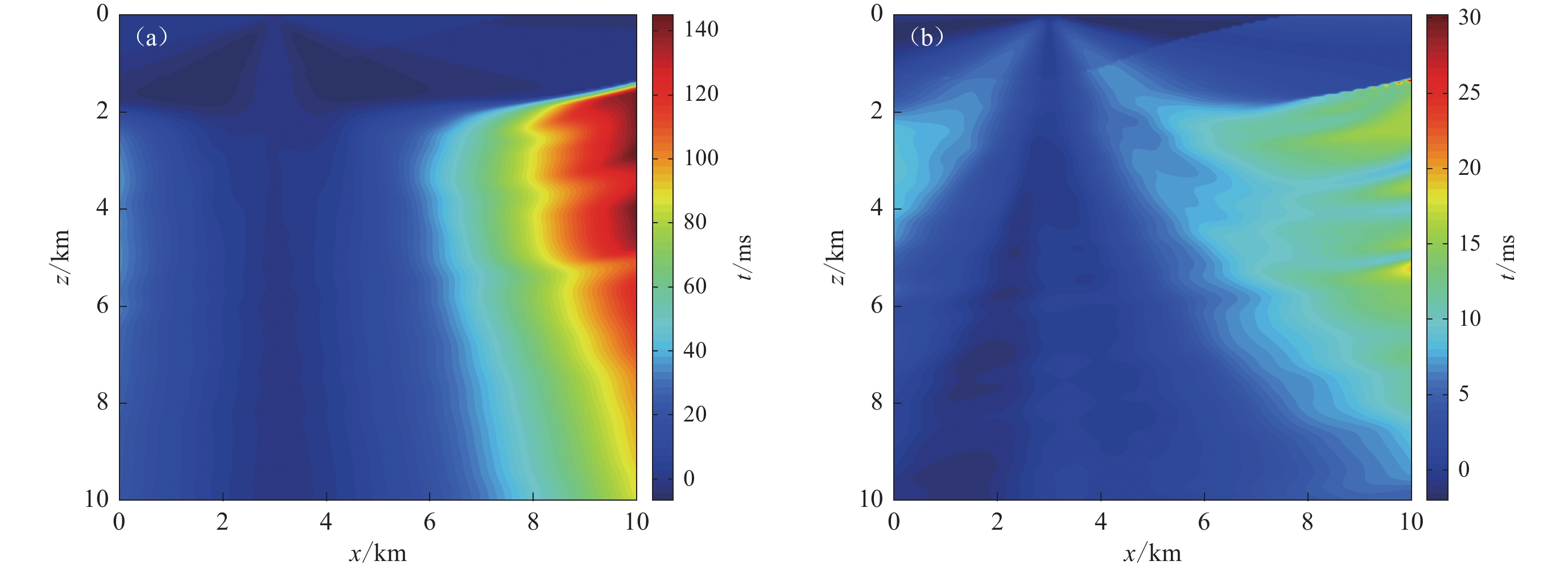
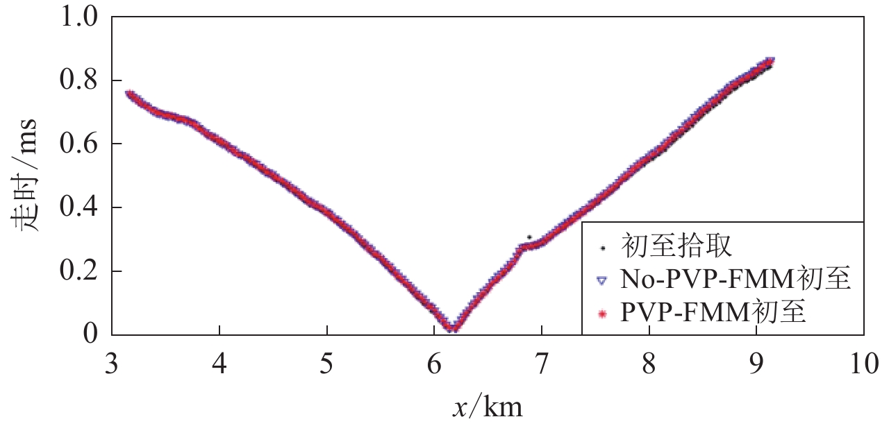
图 12 近地表模型(a) 速度模型;(b) 倾角模型;(c) δ模型;(d) ε模型Figure 12. Near-surface models(a) Velocity;(b) Dip model;(c) δ model;(d) ε model为了与各向同性的FMM进行比较,对该模型分别使用各向同性和各向异性的波场进行有限差分法数值模拟,图13显示的是模拟各向异性介质的一个单炮记录。分别使用各向同性FMM、各向异性No-PVP-FMM和PVP-FMM方法对模型进行射线追踪,图14显示了各向异性模型任意一炮的计算初至与拾取初至的对比图,从图中可以看出,No-PVP-FMM和PVP-FMM的计算初至与从数值模拟中拾取的初至,除了在接近7 km处存在一个异常点之外,几乎全部重合。
![]() 图 14 各向异性模型的计算初至与拾取初至(单炮)Figure 14. First arrival and picked-first arrival calculated by the anisotropic model (single shot)
图 14 各向异性模型的计算初至与拾取初至(单炮)Figure 14. First arrival and picked-first arrival calculated by the anisotropic model (single shot)图15给出了模拟波场初至拾取的结果。图中上部显示的是多个震源的初至时间随偏移距变化的曲线图。横坐标为测线距离,纵坐标为走时。下部是初至时间的炮点和接收点位置。从图中可观测到,与各向同性的初至时间相比,各向异性更小,二者有明显差异。本文方法计算结果与波动方程的有限差分模拟结果具有几乎相同的初至时间。个别异常的走时值源于初至拾取时产生的误差。
![]() 图 15 各向同性(a)和各向异性(b)数值模拟记录拾取的初至时间Figure 15. First arrival time picked up from isotropic (a) and anisotropic (b) numerical simulation records
图 15 各向同性(a)和各向异性(b)数值模拟记录拾取的初至时间Figure 15. First arrival time picked up from isotropic (a) and anisotropic (b) numerical simulation records为了更深入地分析方法的计算误差,本文对比了所有地震道的计算结果与拾取时间的误差,结果如图16所示,可以看出,各向同性与各向异性的误差平均值和方差具有相同的量级,误差分布也相近。
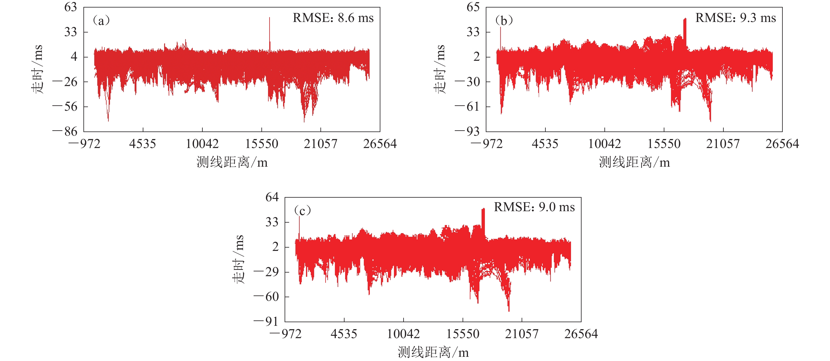
![]() 图 16 射线追踪拟合的误差(913炮)(a) 各向同性FMM射线追踪拟合;(b) 各向异性No-PVP-FMM射线追踪拟合;(c) PVP-FMM射线追踪拟合Figure 16. Error of ray tracing fitting (913 shots)(a) Isotropic FMM ray tracing fitting;(b) Anisotropic No-PVP-FMM ray tracing fitting;(c) PVP-FMM ray tracing fitting
图 16 射线追踪拟合的误差(913炮)(a) 各向同性FMM射线追踪拟合;(b) 各向异性No-PVP-FMM射线追踪拟合;(c) PVP-FMM射线追踪拟合Figure 16. Error of ray tracing fitting (913 shots)(a) Isotropic FMM ray tracing fitting;(b) Anisotropic No-PVP-FMM ray tracing fitting;(c) PVP-FMM ray tracing fitting为了进一步量化分析方法的性能,对913炮的各向同性FMM、各向异性No-PVP-FMM和PVP-FMM的计算误差和计算时间进行统计分析,表1列出了三种方法的计算效率和统计误差。从表中可以看出,三种方法具有相同量级的计算误差。误差均值都很小,各向同性FMM、各向异性No-PVP-FMM和PVP-FMM均方根误差分别为8.6 ms,9.3 ms和9.0 ms,No-PVP-FMM比各向同性方法的增加了0.7 ms,而PVP-FMM仅增加了0.4 ms,比No-PVP-FMM减少了43%。使用2.4 GHz CPU的计算机进行射线追踪,三种方法913炮的总耗时分别为326 s,359 s和372 s。由于No-PVP-FMM增加了群速度计算环节,耗时比各向同性FMM增加10%,而PVP-FMM又添加了相速度预测环节,耗时增加了14%。本文方法与各向同性的FMM具有相同量级计算效率,对于近地表模型同样具有良好的适应性和稳定性。
表 1 三种方法的计算精度和计算效率Table 1. Calculation accuracy and efficiency of the three methods算法 平均误差/ms 均方根误差/ms CPU计算时间/s 各向同性FMM −1.12 8.6 326 No-PVP-FMM −0.03 9.3 359 PVP-FMM −0.16 9.0 372 由以上数值算例可知,本文方法对于不同速度结构模型具有良好的适应性。从Marmousi以及VTI模型中可看出,PVP-FMM方法误差更小,具有更高的走时计算精度。在计算效率方面,虽然PVP-FMM在No-PVP-FMM计算群速度环节的基础上增加了相速度预测环节,但耗时也仅比各向同性FMM增加了14%。此外,本文所提出的方法适用于非均匀TTI介质,因为在均匀介质中,各节点的速度相同,本文所给出的相速度预测公式不起作用。
4. 结论
本文给出的TTI介质的相速度预测公式和PVP-FMM各向异性射线追踪方法,继承了各向同性FMM快速稳定的特点,具有与各向同性FMM相同量级的计算精度。通过理论模型、VTI模型和Marmousi模型测试,验证了本文方法具有小的计算误差和良好的稳定性,能够适用于复杂构造的射线追踪。通过复杂近地表多源模型测试,验证了本文方法的计算结果与有限差分模拟的波场时间能够很好地拟合,在提高FMM走时计算精度的同时,耗时也仅比各向同性FMM增加了14%。
-
![]()
图 12 近地表模型
(a) 速度模型;(b) 倾角模型;(c) δ模型;(d) ε模型
Figure 12. Near-surface models
(a) Velocity;(b) Dip model;(c) δ model;(d) ε model
![]()
图 1 快速推进法(FMM)实现原理图
Figure 1. Implementation schematic diagram of fast marching method (FMM)
![]()
图 3 均匀模型走时及误差对比
(a) 走时对比;(b) 走时绝对误差对比
Figure 3. Comparison of travel time and its error for homogeneous model
(a) Comparison of travel time;(b) Comparison of absolute error of travel time
![]()
图 4 TTI模型走时之差对比
(a) 速度模型;(b) PVP-FMM与No-PVP-FMM走时之差
Figure 4. Comparison of travel time difference for TTI model
(a) Velocity model;(b) Travel time difference between PVP-FMM and No-PVP-FMM
![]()
图 5 利用本文方法PVP-FMM计算所得的射线追踪过程(炮点位于模型中心)
(a) 波前时间场;(b) 相速度矢量场;(c) 群速度矢量场;(d) 射线路径
Figure 5. The ray tracing process calculated by PVP-FMM in this paper (the shot point is located in the center of the model)
(a) Wave front time field;(b) Phase velocity vector field;(c) Group velocity vector field; (d) Ray path
![]()
图 6 VTI模型追踪结果
(a) 速度模型;(b) 波前等时线及射线追踪
Figure 6. Ray tracing results of VTI model
(a) Velocity model;(b) Wavefront isochron and ray path
![]()
图 8 走时绝对误差图
Figure 8. Comparison of absolute error of travel time
(a) No-PVP-FMM;(b) PVP-FMM
![]()
图 9 Marmousi模型追踪结果
(a) 速度模型;(b) 波前等时线及射线追踪
Figure 9. Ray tracing results of Marmousi model
(a) Velocity model;(b) Wavefront isochron and ray path
![]()
图 10 走时等值线对比图
(a) 走时对比;(b) 局部放大图
Figure 10. Comparison map of travel time contour
(a) Comparison of travel time;(b) Local enlarged image
![]()
图 11 走时绝对误差图
Figure 11. Comparison of absolute error of travel time
(a) No-PVP-FMM;(b) PVP-FMM
![]()
图 14 各向异性模型的计算初至与拾取初至(单炮)
Figure 14. First arrival and picked-first arrival calculated by the anisotropic model (single shot)
![]()
图 15 各向同性(a)和各向异性(b)数值模拟记录拾取的初至时间
Figure 15. First arrival time picked up from isotropic (a) and anisotropic (b) numerical simulation records
![]()
图 16 射线追踪拟合的误差(913炮)
(a) 各向同性FMM射线追踪拟合;(b) 各向异性No-PVP-FMM射线追踪拟合;(c) PVP-FMM射线追踪拟合
Figure 16. Error of ray tracing fitting (913 shots)
(a) Isotropic FMM ray tracing fitting;(b) Anisotropic No-PVP-FMM ray tracing fitting;(c) PVP-FMM ray tracing fitting
表 1 三种方法的计算精度和计算效率
Table 1 Calculation accuracy and efficiency of the three methods
算法 平均误差/ms 均方根误差/ms CPU计算时间/s 各向同性FMM −1.12 8.6 326 No-PVP-FMM −0.03 9.3 359 PVP-FMM −0.16 9.0 372  下载: 导出CSV
-
邴琦,孙章庆,韩复兴,王生奥. 2020. 地震波射线追踪方法综述:方法、分类、发展现状与趋势[J]. 地球物理学进展,35(2):536–547. doi: 10.6038/pg2020DD0003 Bing Q,Sun Z Q,Han F X,Wang S A. 2020. Review on the seismic wave ray tracing:Methods,classification,developmental present and trend[J]. Progress in Geophysics,35(2):536–547 (in Chinese).
邓怀群,刘雯林,赵正茂. 2000. 横向各向同性介质中纵波和转换横波的快速射线追踪方法[J]. 石油物探,39(4):1–11. doi: 10.3969/j.issn.1000-1441.2000.04.001 Deng H Q,Liu W L,Zhao Z M. 2000. Fast ray-tracing method for compressional and converted waves in transversely isotropic media[J]. Geophysical Prospecting for Petroleum,39(4):1–11 (in Chinese).
王东鹤,陈祖斌,刘昕,李娜. 2016. 地震波射线追踪方法研究综述[J]. 地球物理学进展,31(1):344–353. doi: 10.6038/pg20160140 Wang D H,Chen Z B,Liu X,Li N. 2016. Review of the seismic ray tracing method[J]. Progress in Geophysics,31(1):344–353 (in Chinese).
张美根,程冰洁,李小凡,王妙月. 2006. 一种最短路径射线追踪的快速算法[J]. 地球物理学报,49(5):1467–1474. doi: 10.3321/j.issn:0001-5733.2006.05.026 Zhang M G,Cheng B J,Li X F,Wang M Y. 2006. A fast algorithm of shortest path ray tracing[J]. Chinese Journal of Geophysics,49(5):1467–1474 (in Chinese).
赵爱华,张美根,丁志峰. 2006. 横向各向同性介质中地震波走时模拟[J]. 地球物理学报,49(6):1762–1769. doi: 10.3321/j.issn:0001-5733.2006.06.024 Zhao A H,Zhang M G,Ding Z F. 2006. Seismic traveltime computation for transversely isotropic media[J]. Chinese Journal of Geophysics,49(6):1762–1769 (in Chinese).
赵烽帆,马婷,徐涛. 2014. 地震波初至走时的计算方法综述[J]. 地球物理学进展,29(3):1102–1113. doi: 10.6038/pg20140313 Zhao F F,Ma T,Xu T. 2014. A review of the travel-time calculation methods of seismic first break[J]. Progress in Geophysics,29(3):1102–1113 (in Chinese).
赵后越,张美根. 2014. 起伏地表条件下各向异性地震波最短路径射线追踪[J]. 地球物理学报,57(9):2910–2917. doi: 10.6038/cjg20140916 Zhao H Y,Zhang M G. 2014. Tracing seismic shortest path rays in anisotropic medium with rolling surface[J]. Chinese Journal of Geophysics,57(9):2910–2917 (in Chinese).
周洪波,张关泉. 1994. 复杂构造区域的初至波走时计算[J]. 地球物理学报,37(4):515–520. doi: 10.3321/j.issn:0001-5733.1994.04.011 Zhou H B,Zhang G Q. 1994. Accurate calculation of first-arrival traveltime in the complex areas[J]. Chinese Journal of Geophysics,37(4):515–520 (in Chinese).
Alkhalifah T. 2000. An acoustic wave equation for anisotropic media[J]. Geophysics,65(4):1239–1250. doi: 10.1190/1.1444815
Fehler M,Keliher P J. 2011. SEAM PhaseⅠ :Challenges of Subsalt Imaging in Tertiary Basins,With Emphasis on Deepwater Gulf of Mexico[M]. Tulsa,Oklahoma:Society of Exploration Geophysicists:1−168.
Garabito G. 2021. Prestack seismic data interpolation and enhancement with common-reflection-surface-based migration and demigration[J]. Geophys Prospect,69(5):913–925. doi: 10.1111/1365-2478.13074
Grechka V,De La Pena A,Schisselé-Rebel E,Auger E,Roux P F. 2015. Relative location of microseismicity[J]. Geophysics,80(6):WC1–WC9. doi: 10.1190/geo2014-0617.1
Hao Q,Waheed U,Alkhalifah T. 2018. A fast sweeping scheme for P-wave traveltimes in attenuating VTI media[C]//Proceedings of the 80th EAGE Conference and Exhibition. Copenhagen,Denmark:EAGE:1−5.
Julian B R,Gubbins D. 1977. Three-dimensional seismic ray tracing[J]. J Geophys,43(1):95–113.
Klibanov M V,Li J Z,Zhang W L. 2023. Numerical solution of the 3-D travel time tomography problem[J]. J Comput Phys,476:111910. doi: 10.1016/j.jcp.2023.111910
Le Bouteiller P,Benjemaa M,Métivier L,Virieux J. 2019. A discontinuous Galerkin fast-sweeping Eikonal solver for fast and accurate traveltime computation in 3D tilted anisotropic media[J]. Geophysics,84(2):C107–C118. doi: 10.1190/geo2018-0555.1
Lelièvre P G,Farquharson C G,Hurich C A. 2011. Computing first-arrival seismic traveltimes on unstructured 3-D tetrahedral grids using the Fast Marching Method[J]. Geophys J Int,184(2):885–896. doi: 10.1111/j.1365-246X.2010.04880.x
Nakanishi I,Yamaguchi K. 1986. A numerical experiment on nonlinear image reconstruction from first-arrival times for two-dimensional island arc structure[J]. J Phys Earth,34(2):195–201. doi: 10.4294/jpe1952.34.195
Sethian J A. 1999. Fast marching methods[J]. SIAM Rev,41(2):199–235. doi: 10.1137/S0036144598347059
Sethian J A,Vladimirsky A. 2003. Ordered upwind methods for static Hamilton-Jacobi equations:Theory and algorithms[J]. SIAM J Numer Anal,41(1):325–363. doi: 10.1137/S0036142901392742
Sun H,Sun J G,Sun Z Q,Han F X,Liu Z Q,Liu M C,Gao Z H,Shi X L. 2017. Joint 3D traveltime calculation based on fast marching method and wavefront construction[J]. Appl Geophys,14(1):56–63. doi: 10.1007/s11770-017-0611-3
Thomsen L. 1986. Weak elastic anisotropy[J]. Geophysics,51(10):1954–1966. doi: 10.1190/1.1442051
Treister E,Haber E. 2016. A fast marching algorithm for the factored Eikonal equation[J]. J Comput Phys,324:210–225. doi: 10.1016/j.jcp.2016.08.012
Tro S,Evans T M,Aslam T D,Lozano E,Culp D B. 2023. A second-order distributed memory parallel fast sweeping method for the Eikonal equation[J]. J Comput Phys,474:111785. doi: 10.1016/j.jcp.2022.111785
Vidale J. 1988. Finite-difference calculation of travel times[J]. Bull Seismol Soc Am,78(6):2062–2076.
Waheed U B,Yarman C E,Flagg G. 2015. An iterative,fast-sweeping-based Eikonal solver for 3D tilted anisotropic media[J]. Geophysics,80(3):C49–C58. doi: 10.1190/geo2014-0375.1
Waheed U B,Alkhalifah T. 2017. A fast sweeping algorithm for accurate solution of the tilted transversely isotropic Eikonal equation using factorization[J]. Geophysics,82(6):WB1–WB8. doi: 10.1190/geo2016-0712.1
Waheed U B. 2020. A fast-marching Eikonal solver for tilted transversely isotropic media[J]. Geophysics,85(6):S385–S393. doi: 10.1190/geo2019-0799.1
Zhao H K. 2004. A fast sweeping method for Eikonal equations[J]. Math Comput,74(250):603–627. doi: 10.1090/S0025-5718-04-01678-3
Zhou B,Greenhalgh S A. 2005. ‘Shortest path’ ray tracing for most general 2D/3D anisotropic media[J]. J Geophys Eng,2(1):54–63. doi: 10.1088/1742-2132/2/1/008


计量
- 文章访问数: 3
- HTML全文浏览量: 1
- PDF下载量: 1
