

Coseismic response of water level in Xin10 well caused by MS6.7 Akto, Xinjiang, earthquake
-
摘要: 本文根据新10井数字化高频采样水位仪记录到的2016年11月25日新疆阿克陶MS6.7地震所引起的水震波,对比分析了该井水位与地表垂向运动的相关性特征,并对二者与井-含水层系统水文参数的关系进行了深入探讨.分析结果显示:①与地震波信号相似,新疆阿克陶MS6.7地震引起的新10井水震波存在两个显著的周期,即6—10 s和15—30 s;②新10井水震波响应幅度与地表垂向运动幅度整体呈正相关,且在高频阶段(频率大于0.08 Hz)二者的振幅比随着频率的减小而增大,表明该井水位对周期大于12 s的信号放大效能较高;③利用水震波与地震波的振幅比估算新10井观测含水层渗透系数的量级为10-2 cm/s,且在地震波作用过程中含水层的水文参数也存在波动.本研究表明,井水位的同震响应机理较为复杂,在分析水位同震响应特征时,高采样率的水位数据是获得可靠结果与认识的基础.
-
关键词:
- 新疆阿克陶MS6.7地震 /
- 水震波 /
- 地震波 /
- 同震响应机理
Abstract: A hydroseismogram induced by the Akto MS6.7 earthquake in Xinjiang on November 25, 2016 was recorded by digital high frequency sampling level gauge. We comparatively analyzed the correlation characteristics between the water level and the vertical ground motion, and the relationship between the above two and the hydrological parameters of well-aquifer system was carried out by a thorough discussion. The results suggested that: ① similar to the seismic signal, there are two significant periods, 6--10 s and 15--30 s in the hydroseismogram of Xin10 well induced by the Akto MS6.7 earthquake. ② overall, the response amplitude of hydroseismogram in Xin10 well was positively correlated to the amplitude of vertical ground motion, and the amplitude ratio of the two increased with the reduction in frequency at high frequency (greater than 0.08 Hz), which indicated that the water level of Xin10 well could enlarge signals with period more than 12 s more effectively. ③ permeability coefficient of Xin10 well-aquifer system was estimated at about 10-2 cm/s by using the amplitude ratio of the hydroseismogram and seismic waves, and the hydrogeological parameters in aquifer also fluctuated during the process of seismic wave action. The results in this paper also showed that the coseismic response mechanism of well water level is more complicated, and high sampling rate of water level data is the guarantee to obtain reliable results and knowledge in coseismic response of water level analysis. -
引 言
以二氧化碳(CO2)为代表的人类温室气体排放引起的气候增温长期成为全球关注焦点。据政府间气候变化专门委员会(IPCC)报告预测,全球地表平均气温到2050年将比1850—1900年平均气温增加约2 ℃ (Pörtner et al,2022)。为此,许多国家提出了碳中和目标和“零碳”方案,其中CO2地质埋存(geological CO2 sequestration,缩写为GCS)是实现这一方案的主要途径(Onarheim et al,2015;Xie et al,2015,2016;Moe,Rottereng,2018;Mishra et al,2019;Zakkour,Heidug,2019;Ciotta et al,2021;Bokka et al,2022)。作为“巴黎协定”的签约国,中国于2020年宣布2030年以前实现“碳达峰”,2060年实现CO2净零排放(Zhou et al,2018;Zhang et al,2022)。据粗略估算,要实现这一目标,我国年平均碳减排量至少需要达到1 Gt以上(Yang et al,2020),这意味着年埋存量百万吨级别以上的大规模和超大规模的GCS实施在不久的将来会很快成为必须面对的现实课题。然而,大规模GCS工程的最大风险是注入引起的盖层破坏和断层滑动诱发的地震(Vilarrasa et al,2013,2016,2023)。也正因为如此,近十年来,GCS有关的断层活化和诱发地震研究逐渐成为热点(Rutqvist et al,2016)。虽然出于埋存效率和安全考虑,GCS项目的选址会尽可能远离活动断层,但对于大规模GCS项目,储层压力的扰动范围可达数百千米以上(Birkholzer et al,2009)。这种空间尺度的断裂勘测在现实中存在巨大挑战,因此总是存在隐伏断裂未被发现的可能性。随着注入的持续,压力增量最终会波及这些亚地震断层,从而影响断层的稳定(Streit,Hillis,2004)。
CO2注入引起的岩石力学效应在GCS安全和环境问题中可能扮演着非常重要的角色(Streit,Hillis,2004;Ferronato et al,2010;Preisig,Prevost,2011;Teatini et al,2014)。多项研究(Parotidis and Shapiro,2004;Rinaldi et al,2019)表明,压力抬升导致有效应力减小进而发生剪切破坏是GCS诱发地震的主要原因。为避免临界应力状态的发生,必须充分了解注入引起的流固(HM)耦合(Streit and Hillis,2004;Vilarrasa et al,2010;Kim and Hosseini,2015;Figueiredo et al,2015),以避免引起诸如CO2泄漏或可感诱发地震等地质力学问题(Rutqvist and Oldenburg,2007;Vilarrasa and Carrera,2015)。因此,从埋存安全和项目可持续的角度考虑,评估储层孔隙压力增量引起的断层复活,预测断层诱发地震震级,进而优化GCS选址和运营方案是大规模GCS实施亟需解决的问题。尽管数值模拟无疑是评估GCS上述问题的重要手段。然而,现实中数值模拟的计算效率对于复杂的HM问题常常不尽人意。相比而言,利用已经验证的解析解去分析和评估CO2注入引起的上述复杂过程则简便高效得多,有利于风险管控和灾害预警。现有岩石力学解析研究(Jansen et al,2019;Wu et al,2021;Jansen and Meulenbroek,2022)均只针对一条断裂的地质模型进行公式推导,目前还未见有研究报道多断裂型储层的孔隙弹性场解析解。构造运动一般不可能只产生单条断裂,更多的情况是沿着平行或垂直于最大主应力方向发育一组或多组断裂(侯泉林等,2018)。然而,目前关于诱发地震的研究也都是基于单条发震断层的力学分析(Vilarrasa et al,2023; Wu et al,2022,2023)。开展多井(多场地)注入的大规模GCS也很难避免储层在区域上被多条断层切割的情形。因此,基于多断层切穿型储层模型,发展CO2注入问题的力学解析解,几乎是大规模GCS计划刻不容缓的首要问题。只有这个问题得到解决,大规模GCS带来的安全问题才更有科学保障,有利于注入方案的优化和诱发地震的管理。基于上述考虑,本研究在总结现有解析解的基础上,发展并提出一套完整的解析工具,用以评估盆地尺度的大规模CO2注入引起的储层安全和断层稳定性。研究成果将为我国GCS远景盆地的大规模实施提供安全性评估范例和方案优选建议。
1. 问题与几何模型
为适应多场地尺度(盆地尺度)大规模GCS工程的注入安全和地震评估需求,本研究将前人(Jansen et al,2019;Wu et al,2021)的概念模型(图1A)扩展至三条断层(图1B),坐标系原点设在注入中心(单井时为注入井位置,多井时为注入井井群的几何中心)。模型范围在xz平面上无限延伸,而在y平面上为单位长度。图中的储层尺寸、断层位置、几何参数、水力性质均为用户可灵活设定的值;图中所示的压力锋(即:红色填充区的左右侧边界)则仅代表某时刻的特定位置,它实际是从注入中心随时间向外推进的。基于图1B所示模型,我们应用夹杂理论(Eshelby,1957,1959)推导储层孔隙压力变化引起的线弹性位移、应变和应力。
![]() 图 1 A前人研究与B本研究几何模型的对比Figure 1. Comparison of the conceptual models between A previous studies and B the present study
图 1 A前人研究与B本研究几何模型的对比Figure 1. Comparison of the conceptual models between A previous studies and B the present study夹杂理论是细观乃至微观力学的学科基石。所谓“夹杂”(inclusion)是指材料中弹性参数区别于基体的杂质体(张向宁,2020)。该理论的实质是Eshelby (1957,1959)为求解无限大基体中单个椭球夹杂的弹性场而提出的等效夹杂方法。该方法假设基体与夹杂具有相同弹性行为,但只有夹杂受均匀本征应变(非弹性应变)作用。等效夹杂方法求解Eshelby夹杂问题的步骤有三:(1) 将夹杂从基体中取出并允许其自由膨胀变形;(2) 在夹杂表面施加适当面力使其恢复原形和体积,然后将夹杂重新放入基体中原本的位置并与基体相接;(3) 释放夹杂面力,夹杂对基体的作用力大小等于夹杂表面施加的面力,但作用方向相反。
格林函数又称为点源影响函数,是数学物理中的一个重要概念,它代表一个点源在一定边界条件和初始条件下所产生的场。格林函数法是求解数学物理方程的常用方法之一。弹性力学中引入格林函数求解弹性复合固体(即:夹杂问题)的位移场和应力场。格林函数是通过求解弹性平衡方程在给定边界条件下的狄拉克δ函数力而获得的。
2. CO2注入引起的孔隙压力增量和孔隙弹性解析解
2.1 孔隙压力增量
单井注入条件下的储层孔隙压力增量采用De Simone and Krevor (2021)提出的解析解进行计算。假设CO2体积注入速率为Q,含水层水平展布半径为Rres,厚度为H,水平绝对渗透率为k,则t时刻距离注入中心r处的压力增量∆P等于:
$$ \Delta P ( r\text{,} t ) =\dfrac{Q t \mu_{w}}{2 \pi k H \rho_{c}} {{×}}\left\{\begin{array}{l} \dfrac{\mu_{c}}{\mu_{w}} \ln \left(\dfrac{\psi}{r}\right) +\ln \left(\dfrac{R_{\text {res}}}{\psi}\right)+C_{b}\text{,} r{{<}}\psi \\ \ln \left(\dfrac{R_{r e s}}{\psi}\right) +C_{b}\text{,} \qquad \qquad \quad \psi {{<}}r{{<}}R_{\text {res }} \\ 0\text{,} \qquad \qquad \qquad \qquad \quad \quad r{{>}}R_{\text {res }} \end{array}\right. $$ (1) 上式中$ \psi=\mathrm{e}\mathrm{x}\mathrm{p} ( \omega ) \xi $,其中$ \omega=\dfrac{{\mu }_{c} +{\mu }_{w}}{ ( {\mu }_{c}-{\mu }_{w} ) }\mathrm{ln}\left( \sqrt{\dfrac{{\mu }_{c}}{{\mu }_{w}}}\right) -1 $,μw和μc分别为水和CO2的动力黏度, ρc为CO2的密度,$ \xi=\sqrt{Qt/ ( \pi \varphi H{\rho }_{c} ) } $;Cb的定义如下:
$$ C_{b}=\left\{\begin{array}{ll} 0\text{,} &R{{<}}=R_{\text {res }} \\ \dfrac{2 R^{2}}{2.25 R_{c}^{2}}-\dfrac{3}{4} \text{,} & R {{<}}R_{\text {res }} \end{array}\right. $$ (2) 压力扰动半径$ R=\sqrt{2.25kt/ ( {\mu }_{w}\beta ) } $,其中β为含水层总压缩系数。对于多井并注情形,若井数为n,则ri处与第j口井相距dij的孔隙压力增量由叠加原理可得:
$$ \Delta P_{\text {sup }} ( r_{i}\text{,} t ) =\sum_{j=1}^{n} \Delta P ( d_{i j}\text{,} t ) $$ (3) 2.2 地动位移
基于地层岩石的线弹性力学假设,应用夹杂理论(Eshelby,1957,1959)可计算复杂几何夹杂域内某点的点力引起某场点的位移。Jansen et al.(2019) 和Cornelissen et al.(2024)先后都给出了二维平面应变条件下矩形和三角形夹杂孔隙压力变化引起的线弹性位移解析解,他们利用自己的解析解评估了单条断裂切割型储层的地动位移。然而,他们的解均将坐标原点设定在断层线中点,且只能评估一条断裂。为满足多断层切割型储层CO2注入评估的需要,我们推导了坐标原点偏离断裂、储层被三条断裂切穿情形的线弹性解析解。考虑图1B所示断裂型储层模型,坐标原点位于孔隙压力影响半径的圆心。当影响半径R推进到图中所示的位置时,夹杂域(即:图中粉红色所示压力扰动区)由两个直角梯形和一个梯形组成,而每个梯形又可进一步分解为一个矩形和一个直角三角形(图2)。由线弹性假设可得,格林函数亦可进行线性加减计算。因此,我们首先要做的是,推导当夹杂域几何形状分别为矩形和四种不同朝向的直角三角形时,域内所有点力(对本研究而言,即孔隙压力抬升产生的本征应力)引起外场某点的位移,即位移格林函数在相应夹杂域几何体上的积分。对于内场(夹杂域内)某点的无量纲位移,只需按外场点计算方法再减去π即可。此方法也同样适用于2.3和2.4节中的应变和应力计算。为节约篇幅,下文我们仅给出外场任意点的解析解。
![]() 图 2 夹杂域几何体分解示例及直角三角形命名Figure 2. An example of decomposition of the geometry of the inclusion domain and the names of right triangles
图 2 夹杂域几何体分解示例及直角三角形命名Figure 2. An example of decomposition of the geometry of the inclusion domain and the names of right triangles据Mura (2013)给出的平面应变条件格林函数,“矩形”在x和z方向的比例位移$G_{x}^{\square} $和$G_{{\textit{z}}}^{\square} $可通过如下格林函数的积分求得:
$$ \begin{split} G_{x}^{\square} =&\int_{r}^{s} \int_{p}^{q} \frac{x-\zeta}{ ( x-\zeta ) ^{2} + ( {\textit{z}} -\xi ) ^{2}} d \zeta d \xi \\ =&\frac{1}{2} \int_{r}^{s} \ln [ ( x-p ) ^{2} + ( {\textit{z}} -\xi ) ^{2} ] d \xi-\frac{1}{2} \int_{r}^{s} \ln [ ( x-q ) ^{2} + ( {\textit{z}} -\xi ) ^{2} ] d \xi \\ =& ( x-p ) \left( a \tan \frac{{\textit{z}} -r}{x-p}-a \tan \frac{{\textit{z}} -s}{x-p}\right) + ( x-q ) \left(a \tan \frac{{\textit{z}} -s}{x-q}-a \tan \frac{{\textit{z}} -r}{x-q} \right) \\ &+ \frac{{\textit{z}} -r}{2} \ln \frac{ ( x-p ) ^{2} + ( {\textit{z}} -r ) ^{2}}{ ( x-q ) ^{2} + ( {\textit{z}} -r ) ^{2}} +\frac{{\textit{z}} -s}{2} \ln \frac{ ( x-q ) ^{2} + ( {\textit{z}} -s ) ^{2}}{ ( x-p ) ^{2} + ( {\textit{z}} -s ) ^{2}} \end{split} $$ (4) $$ \begin{split} G_{{\textit{z}} }^{\square} =&\displaystyle\int_{p}^{q} \displaystyle\int_{r}^{s} \frac{{\textit{z}} -\xi}{ ( x-\zeta ) ^{2} + ( {\textit{z}} -\xi ) ^{2}} d \xi d \zeta \\ =&\frac{1}{2} \displaystyle\int_{p}^{q} \ln [ ( x-\zeta ) ^{2} + ( {\textit{z}} -r ) ^{2} ] d \zeta-\frac{1}{2} \displaystyle\int_{p}^{q} \ln [ ( x-\zeta ) ^{2} + ( {\textit{z}} -s ) ^{2} ] d \zeta \\ =& ( {\textit{z}} -r ) \left( a \tan \frac{x-p}{{\textit{z}} -r}-a \tan \frac{x-q}{{\textit{z}} -r}\right) + ( {\textit{z}} -s ) \left(a \tan \frac{x-q}{{\textit{z}} -s}-a \tan \frac{x-p}{{\textit{z}} -s}\right) \\ & +\frac{x-p}{2} \ln \frac{ ( x-p ) ^{2} + ( {\textit{z}} -r ) ^{2}}{ ( x-p ) ^{2} + ( {\textit{z}} -s ) ^{2}} +\frac{x-q}{2} \ln \frac{ ( x-q ) ^{2} + ( {\textit{z}} -s ) ^{2}}{ ( x-q ) ^{2} + ( {\textit{z}} -r ) ^{2}} \end{split} $$ (5) “右下三角形”在x和z方向的无量纲位移$ G_{x}^{\lrcorner} $和$ G_{{\textit{z}} }^{\lrcorner} $可通过如下积分求得:
$$ \begin{aligned} G_{x}^{\lrcorner} =&\displaystyle\int_{r}^{s} \displaystyle\int_{p- ( s-\xi ) \cot \theta}^{p} \frac{x-\zeta}{ ( x-\zeta ) ^{2} + ( {\textit{z}} -\xi ) ^{2}} d \zeta d \xi =\displaystyle\int_{r}^{s} \frac{1}{2} \ln \left\{ [ x-p + ( s-\xi ) \cot \theta ] ^{2} + ( {\textit{z}} -\xi ) ^{2}\right\} d \xi \\ & -\displaystyle\int_{r}^{s} \frac{1}{2} \ln [ ( x-p ) ^{2} + ( {\textit{z}} -\xi ) ^{2} ] d \xi = ( x-p ) \left( a \tan \frac{{\textit{z}} -s}{x-p}-a \tan \frac{{\textit{z}} -r}{x-p}\right) -\frac{{\textit{z}} -r}{2} \ln [ ( x-p ) ^{2} + ( {\textit{z}} -r ) ^{2} ] \\ & -\frac{\sin \theta \cos \theta [ x-p + ( s-{\textit{z}} ) \cot \theta ] }{2} \ln [ ( x-p ) ^{2} + ( {\textit{z}} -s ) ^{2} ] \\ & +\frac{\sin \theta \cos \theta ( x-p ) +s \cos ^{2} \theta +{\textit{z}} \sin ^{2} \theta-r}{2} {{×}} \ln \left\{ [ x-p + ( s-r ) \cot \theta ] ^{2} + ( {\textit{z}} -r ) ^{2}\right\} \\ & +\sin ^{2} \theta [ x-p + ( s-{\textit{z}} ) \cot \theta ] \left\{a \tan \left[\cot \theta +\frac{ ( {\textit{z}} -r ) \csc ^{2} \theta}{x-p + ( s-{\textit{z}} ) \cot \theta}\right] -a \tan \left[\cot \theta +\frac{ ( {\textit{z}} -s ) \csc ^{2} \theta}{x-p + ( s-{\textit{z}} ) \cot \theta}\right]\right\} \end{aligned} $$ (6) $$ \begin{split} G_{{\textit{z}} }^{\lrcorner} =&\int_{p- ( s-r ) \cot \theta}^{p} \int_{r}^{s- ( p-\zeta ) \tan \theta} \frac{{\textit{z}} -\xi}{ ( x-\zeta ) ^{2} + ( {\textit{z}} -\xi ) ^{2}} d \xi d \zeta=\int_{p- ( s-r ) \cot \theta}^{p} \frac{1}{2} \ln [ ( x-\zeta ) ^{2} + ( {\textit{z}} -r ) ^{2} ] d \zeta \\ & -\int_{p- ( s-r ) \cot \theta}^{p} \frac{1}{2} \ln \left\{ ( x-\zeta ) ^{2} + [ ( {\textit{z}} -s ) + ( p-\zeta ) \tan \theta ] ^{2}\right\} d \zeta \\ =& ( {\textit{z}} -r ) \left[a \tan \frac{ ( s-r ) \cot \theta +x-p}{{\textit{z}} -r}-a \tan \frac{x-p}{{\textit{z}} -r}\right] \\ & + [ \sin \theta \cos \theta ( x-p ) + ( s-{\textit{z}} ) \cos ^{2} \theta ] \left[a \tan \frac{ ( {\textit{z}} -s ) \tan \theta +x-p}{ ( x-p ) \tan \theta +s-{\textit{z}} }\right. \\ & \left.-a \tan \frac{ ( {\textit{z}} -r ) \tan \theta + ( x-p ) + ( s-r ) \cot \theta}{ ( x-p ) \tan \theta +s-{\textit{z}} }\right] +\frac{x-p}{2} \ln \frac{ [ x-p + ( s-r ) \cot \theta ] ^{2} + ( {\textit{z}} -r ) ^{2}}{ ( x-p ) ^{2} + ( {\textit{z}} -r ) ^{2}} \\ & +\frac{ ( x-p ) \cos ^{2} \theta +\sin \theta \cos \theta ( {\textit{z}} -s ) }{2} \ln \frac{ ( x-p ) ^{2} + ( {\textit{z}} -s ) ^{2}}{ [ x-p + ( s-r ) \cot \theta]^{2} + ( {\textit{z}} -r ) ^{2} ] } \end{split} $$ (7) 图2所示的剩余三种直角三角形夹杂在x和z方向的比例位移格林函数积分见本文附录(式(A.1)—式(A.6))。假设当地大气压为Pa,在地层静水压力假设条件下,当z=(P0−Pa)/(ρg)时,代入上述公式可近似估算地表位移。上述格林函数(式(4)—式(7)及式(A.1)—式(A.6))表征的是比例地动位移,实际的地动位移需乘以位移比例因子Du:
$$ {D}_{u}=\frac{ ( 1-2\nu ) \alpha \Delta {P}_{inc}}{2\pi ( 1-\nu ) G} $$ (8) 上式中ν为泊松比;α为Biot系数(也即有效应力系数);ΔPinc为储层平均孔隙压力增量;G为剪切模量。
2.3 应变增量
平面应变条件下,对积分形式的位移格林函数求空间偏导,再依据协调性方程即得到比例化总应变张量。为编程方便和书写简洁起见,我们对每种几何形态的夹杂域分别定义了七个辅助函数。
以“右下三角形”为例,其对应的三个比例应变分量分别为:
$$ \begin{split} &f_{1}^{\lrcorner} ( x\text{,} {\textit{z}} \text{,} p\text{,} s\text{,} \theta\text{,} \hat{{\textit{z}} } ) = [ x-p + ( s-\hat{{\textit{z}} } ) \cot \theta ] ^{2} + ( {\textit{z}} -\hat{{\textit{z}} } ) ^{2} \\& f_{2}^{\lrcorner} ( x\text{,} {\textit{z}} \text{,} p\text{,} s\text{,} \theta\text{,} \hat{{\textit{z}} } ) = ( x-p ) \cot \theta +{\textit{z}} -s + ( s-\hat{{\textit{z}} } ) \csc ^{2} \theta \\& f_{3}^{\lrcorner} ( x\text{,} {\textit{z}} \text{,} p\text{,} s\text{,} \theta\text{,} \hat{{\textit{z}} } ) = [ x-p + ( s-\hat{{\textit{z}} } ) \cot \theta ] \dfrac{f_{2}^{\lrcorner} ( x\text{,} {\textit{z}} \text{,} p\text{,} s\text{,} \theta\text{,} \hat{{\textit{z}} } ) }{f_{1}^{\lrcorner} ( x\text{,} {\textit{z}} \text{,} p\text{,} s\text{,} \theta\text{,} \hat{{\textit{z}} } ) } \\& f_{4}^{\lrcorner} ( x\text{,} {\textit{z}} \text{,} p\text{,} s\text{,} \theta\text{,} \hat{{\textit{z}} } ) =\dfrac{{\textit{z}} -{\textit{z}} }{f_{1}^{\lrcorner} ( x\text{,} {\textit{z}} \text{,} p\text{,} s\text{,} \theta\text{,} {\textit{z}} ) + ( f_{2}^{\lrcorner} ) ^{2} ( x\text{,} {\textit{z}} \text{,} p\text{,} s\text{,} \theta\text{,} \hat{{\textit{z}} } ) } \\& f_{5}^{\lrcorner} ( x\text{,} {\textit{z}} \text{,} p\text{,} s\text{,} \theta\text{,} \hat{{\textit{z}} } ) =a \tan \left[\cot \theta +\dfrac{ ( {\textit{z}} -\hat{{\textit{z}} } ) \csc ^{2} \theta}{x-p + ( s-{\textit{z}} ) \cot \theta}\right] \\& f_{6}^{\lrcorner} ( x\text{,} {\textit{z}} \text{,} p\text{,} s\text{,} \theta\text{,} \hat{{\textit{z}} } ) =\dfrac{ ( {\textit{z}} -\hat{{\textit{z}} } ) f_{2}^{\lrcorner} ( x\text{,} {\textit{z}} \text{,} p\text{,} s\text{,} \theta\text{,} \hat{{\textit{z}} } ) }{f_{1}^{\lrcorner} ( x\text{,} {\textit{z}} \text{,} p\text{,} s\text{,} \theta\text{,} \hat{{\textit{z}} } ) } \\& f_{7}^{\lrcorner} ( x\text{,} {\textit{z}} \text{,} p\text{,} s\text{,} \theta\text{,} \hat{{\textit{z}} } ) =\dfrac{x-p + ( s-\hat{{\textit{z}} } ) \cot \theta}{f_{1}^{\lrcorner} ( x\text{,} {\textit{z}} \text{,} p\text{,} s\text{,} \theta\text{,} {\textit{z}} ) + ( f_{2}^{\lrcorner} ) ^{2} ( x\text{,} {\textit{z}} \text{,} p\text{,} s\text{,} \theta\text{,} \hat{{\textit{z}} } ) } \end{split} $$ (9) $$ \begin{split} G_{x x}^{\lrcorner}=&\frac{\partial G_{x}^{\lrcorner}}{\partial x} =\sin ^{2} \theta [ f_{3}^{\lrcorner} ( x\text{,} {\textit{z}} \text{,} p\text{,} s\text{,} \theta\text{,} r ) -f_{3}^{\lrcorner} ( x\text{,} {\textit{z}} \text{,} p\text{,} s\text{,} \theta\text{,} s ) ] +a \tan \frac{{\textit{z}} -s}{x-p} \\ & -a \tan \frac{{\textit{z}} -r}{x-p} +\frac{\sin \theta \cos \theta}{2} \ln \frac{f_{1}^{\lrcorner} ( x\text{,} {\textit{z}} \text{,} p\text{,} s\text{,} \theta\text{,} r ) }{f_{1}^{\lrcorner} ( x\text{,} {\textit{z}} \text{,} p\text{,} s\text{,} \theta\text{,} s ) } \\ & + [ x-p + ( s-{\textit{z}} ) \cot \theta ] [ f_{4}^{\lrcorner} ( x\text{,} {\textit{z}} \text{,} p\text{,} s\text{,} \theta\text{,} s ) -f_{4}^{\lrcorner} ( x\text{,} {\textit{z}} \text{,} p\text{,} s\text{,} \theta\text{,} r ) ] \\ & +\sin ^{2} \theta [ f_{5}^{\lrcorner} ( x\text{,} {\textit{z}} \text{,} p\text{,} s\text{,} \theta\text{,} r ) -f_{5}^{\lrcorner} ( x\text{,} {\textit{z}} \text{,} p\text{,} s\text{,} \theta\text{,} s ) ] \end{split} $$ (10) $$ \begin{split} G_{{\textit{z}} {\textit{z}} }^{\lrcorner}&\frac{\partial G_{{\textit{z}} }^{\lrcorner}}{\partial {\textit{z}} } =\sin \theta \cos \theta [ f_{6}^{\lrcorner} ( x\text{,} {\textit{z}} \text{,} p\text{,} s\text{,} \theta\text{,} s ) -f_{6}^{\lrcorner} ( x\text{,} {\textit{z}} \text{,} p\text{,} s\text{,} \theta\text{,} r ) ] +a \tan \frac{x-p + ( s-r ) \cot \theta}{{\textit{z}} -r} \\ & -a \tan \frac{x-p}{{\textit{z}} -r} +\frac{\sin \theta \cos \theta}{2} \ln \frac{f_{1}^{\lrcorner} ( x\text{,} {\textit{z}} \text{,} p\text{,} s\text{,} \theta\text{,} s ) }{f_{1}^{\lrcorner} ( x\text{,} {\textit{z}} \text{,} p\text{,} s\text{,} \theta\text{,} r ) } \\ & + [ ( x-p ) \cot \theta + ( s-{\textit{z}} ) \cot ^{2} \theta ] [ f_{7}^{\lrcorner} ( x\text{,} {\textit{z}} \text{,} p\text{,} s\text{,} \theta\text{,} s ) -f_{7}^{\lrcorner} ( x\text{,} {\textit{z}} \text{,} p\text{,} s\text{,} \theta\text{,} r ) ] \\ & +\cos ^{2} \theta [ f_{5}^{\lrcorner} ( x\text{,} {\textit{z}} \text{,} p\text{,} s\text{,} \theta\text{,} r ) -f_{5}^{\lrcorner} ( x\text{,} {\textit{z}} \text{,} p\text{,} s\text{,} \theta\text{,} s ) ] \end{split} $$ (11) $$ \begin{split} G_{x {\textit{z}} }^{\lrcorner}=&\frac{1}{2}\left(\frac{\partial G_{x}}{\partial {\textit{z}} } +\frac{\partial G_{{\textit{z}} }}{\partial x}\right) =\frac{1}{2} \ln \frac{ ( x-p ) ^{2} + ( {\textit{z}} -s ) ^{2}}{ ( x-p ) ^{2} + ( {\textit{z}} -r ) ^{2}} +\frac{\sin ^{2} \theta}{2} \ln \frac{f_{1}^{\lrcorner} ( x\text{,} {\textit{z}} \text{,} p\text{,} s\text{,} \theta\text{,} r ) }{f_{1}^{\lrcorner} ( x\text{,} {\textit{z}} \text{,} p\text{,} s\text{,} \theta\text{,} s ) } \\ & +\frac{\sin \theta \cos \theta}{2} [ f_{3}^{\lrcorner} ( x\text{,} {\textit{z}} \text{,} p\text{,} s\text{,} \theta\text{,} s ) -f_{3}^{\lrcorner} ( x\text{,} {\textit{z}} \text{,} p\text{,} s\text{,} \theta\text{,} r ) ] \\ & +\frac{1}{2} [ ( x-p ) \cot \theta + ( s-{\textit{z}} ) \cot ^{2} \theta ] [ f_{4}^{\lrcorner} ( x\text{,} {\textit{z}} \text{,} p\text{,} s\text{,} \theta\text{,} r ) -f_{4}^{\lrcorner} ( x\text{,} {\textit{z}} \text{,} p\text{,} s\text{,} \theta\text{,} s ) ] \\ & +\sin \theta \cos \theta [ f_{5}^{\lrcorner} ( x\text{,} {\textit{z}} \text{,} p\text{,} s\text{,} \theta\text{,} s ) -f_{5}^{\lrcorner} ( x\text{,} {\textit{z}} \text{,} p\text{,} s\text{,} \theta\text{,} r ) ] \\ & +\frac{\sin ^{2} \theta}{2} [ f_{6}^{\lrcorner} ( x\text{,} {\textit{z}} \text{,} p\text{,} s\text{,} \theta\text{,} r ) -f_{6}^{\lrcorner} ( x\text{,} {\textit{z}} \text{,} p\text{,} s\text{,} \theta\text{,} s ) ] \\ & +\frac{1}{2} [ x-p + ( s-{\textit{z}} ) \cot \theta ] [ f_{7}^{\lrcorner} ( x\text{,} {\textit{z}} \text{,} p\text{,} s\text{,} \theta\text{,} r ) -f_{7}^{\lrcorner} ( x\text{,} {\textit{z}} \text{,} p\text{,} s\text{,} \theta\text{,} s ) ] \end{split}$$ (12) 图2所示的剩余三种直角三角形所对应的七个辅助函数和三个比例应变分量见本文附录(式(B.1)—式(B.12))。
2.4 应力增量
根据均匀各向同性材料的胡克定律,弹性应变e (等于总应变ϵ减去本征应变ϵ*)与应力σ的关系为σ=λtr(e)+2µe,式中λ和µ分别为拉梅第一参数和拉梅第二参数,tr(e)表示应变张量e的迹。由此我们得到来自j方向的点力在点x处产生的i方向的应力分量,即σij(x)的表达式为
$$ \sigma_{i j} ( \mathbf{x} ) = \lambda\left[\epsilon_{k k} ( \mathbf{x} ) -\epsilon_{k k}^{\star} ( \mathbf{x} ) \right] \delta_{i j} +2 \mu\left[\epsilon_{i j} ( \mathbf{x} ) -\epsilon_{i j}^{\star} ( \mathbf{x} ) \right]=\lambda \delta_{i j} \epsilon_{k k} ( \mathbf{x} ) +2 \mu \epsilon_{i j} ( \mathbf{x} ) -\sigma_{i j}^{\star} ( \mathbf{x} ) $$ (13) 式中δ称为克罗内克函数,定义如下:
$$ \delta_{i j}=\left\{\begin{array}{ll} 1\text{,} & i=j \\ 0\text{,} & i{{≠}} j \end{array}\right. $$ (14) 因此式(13)也可写成如下的张量形式,其中的σ*为本征应力。
$$ \boldsymbol{\sigma}=\lambda [ \operatorname{tr} ( \boldsymbol{\epsilon} ) -\operatorname{tr} ( \boldsymbol{\epsilon}^{\star} ) ] \boldsymbol{\delta} +2 \mu [ \boldsymbol{\epsilon}-\boldsymbol{\epsilon}^{\star} ] =\lambda \boldsymbol{\delta} \operatorname{tr} ( \boldsymbol{\epsilon} ) +2 \mu \boldsymbol{\epsilon}-\boldsymbol{\sigma}^{\star} $$ (15) 2.5 库仑破坏应力
设断层面上的有效正应力和切应力分别为σ′n和τ,静摩擦系数为ηst,采用固体力学中应力正负所表示的物理意义,即σ′n为正表示拉应力,为负表示压应力;τ为正表示切应力指向断盘顺时针转动的方向,为负则表示切应力指向断盘逆时针转动的方向,因此断层面上的库仑破坏应力CFS(King et al,1994;Jansen et al,2019;Wu et al,2021)可定义为
$$ C F S=|\tau| +\eta_{s t} \sigma_{n}^{\prime} $$ (16) 断层稳定性趋势可通过库仑破坏应力的变化∆CFS来评估,即
$$ \Delta C F S ( {\textit{z}} \text{,} t ) =C F S ( {\textit{z}} \text{,} t ) -C F S ( {\textit{z}} \text{,} 0 ) $$ (17) ∆CFS>0意味着断层不稳定趋势增加,即诱发应力促使断层向破坏发展,最终导致同震滑动。反之则表示断层稳定性提高。
2.6 断层滑动段
断层滑动段(xz平面上为若干不连续线段)是指CFS>0的断层部位。因此,根据断层面上的CFS值,我们可以很容易地识别出断层滑动段沿断层倾向或埋深方向的分布。通过计算断层最大滑动段的长度可初步评估CO2注入诱发地震的危害(Wu et al,2021)。
3. CO2注入断裂型储层的力学响应—案例研究
3.1 模型结构及参数
为实现采用第2节所述解析方法评估CO2注入引起的断层稳定性问题,我们编制了由数十个函数构成的PYTHON脚本程序。通过表1所列参数定义了一个典型断陷盆地水平含水层被三条导水正断层(表2)切穿的模型。如第2节已说明的那样,整个计算域(包括含水层、断层和围岩)为一均质各向同性弹性变形域,这意味着断层和围岩的力学性质(摩擦系数除外)与含水层相同。断层厚度为零。初始垂直应力$\sigma ^0_{{\textit{z}} {\textit{z}} } $来自上覆地层自重,负值表示方向朝下。本案例演示的是CO2注入速率Q为0.26 m3/s时的单井作业情形。对于多井并注工况,程序增加了计算多井孔隙压力增量的面积加权平均所需时间,因此通常会比此案例(约6小时)增加几十分钟乃至几个小时(取决于井数多少)。
表 1 含水层几何与物性参数Table 1. Geometric parameters and physical properties of the faulted aquifer参数符号 物理含义 取值 单位 $ {R}_{\mathrm{r}\mathrm{e}\mathrm{s}} $ 含水层水平展布半径 20000 m $ H $ 含水层厚度 300 m $ \varnothing $ 孔隙度 0.15 − $ k $ 水平渗透率 1×10⁻¹⁴ m2 $ {T}_{0} $ 初始温度 50 ℃ $ {P}_{0} $ 初始孔隙压力 20 MPa $ {X}_{\mathrm{s}} $ 盐度 0.01 kg NaCl/kg H2O $ {C}_{\mathrm{r}} $ 孔隙压缩系数 1×10⁻¹⁰ 1/Pa $ \upsilon $ 泊松比 0.15 − $ \alpha $ Biot系数 0.9 − $ G $ 剪切模量 6 500 MPa $ {k}_{\mathrm{e}\mathrm{p}} $ 侧压系数 0.65 − $ {\sigma }_{{\textit{z}} {\textit{z}} }^{0} $ 初始垂直应力 −55 MPa $ {\sigma }_{x{\textit{z}} }^{0} $ 初始剪切应力 0 MPa 表 2 断层几何及水力性质Table 2. Geometry and hydraulic nature of the faults符号 $ {x}_{in} $ $ \theta $ b-a / $ {\eta }_{st} $ 物理意义 断层x轴截距坐标 断层倾角 断距 水力性质 静摩擦系数 单位 m ° m / − F1断层取值 10000 70 100 导水 0.6 F2断层取值 − 6000 140 150 导水 0.7 F3断层取值 15000 50 200 导水 0.5 3.2 孔隙压力增量
CO2注入含水层会造成孔隙流体压力抬升。随着流体的运移,孔隙压力沿注入中心向远井区域扩散。图3给出了采用2.1节所述方法计算的储层孔隙压力增量的时空分布和夹杂域及断层的孔隙压力增量动态。计算结果与我们的预期一致,持续注入条件下,某点的孔隙压力增量随注入时长增加而增加,同一时刻的孔隙压力增量随径向距离增加而减小。由于本算例我们设置的含水层渗透率中等(1×10⁻¹⁴ m2)但注入速率较大(0.26 m3/s,约6 Mt/a),且含水层有界(径向距离为20 km),因此孔隙压力抬升总体较高,连续注入100 年,注入中心处孔隙压力增量约42 MPa (图3A)。采用面积加权平均法得到的夹杂域平均孔隙压力增量代表整个压力扰动区域内的储层孔隙压力平均增量,因此明显小于注入中心附近的孔隙压力增量,也多数时间小于断层中心处的孔隙压力增量(图3B)。注入50年的孔隙压力增量为7 MPa,至100年,孔隙压力增量提升至17 MPa。
![]() 图 3 A. 不同时刻储层孔隙压力增量沿径向距离的分布;B.夹杂域的平均孔隙压力增量和三条断层处的孔隙压力增量Figure 3. A The radial distribution of the incremental pore pressures at various injection times and B Temporal evolution of the inclusion-averaging increase in pore pressure and the incremental pore pressures on the faults
图 3 A. 不同时刻储层孔隙压力增量沿径向距离的分布;B.夹杂域的平均孔隙压力增量和三条断层处的孔隙压力增量Figure 3. A The radial distribution of the incremental pore pressures at various injection times and B Temporal evolution of the inclusion-averaging increase in pore pressure and the incremental pore pressures on the faults3.3 地动位移增量
图4给出了储层深度三条断层附近的比例位移,可见注入使得水平位移集中在断层左右同时与储层和围岩(上覆和下伏地层)接触的埋深段,而垂向位移随深度匀滑递变。由于F1和F3断层为纸面左倾断层,注入导致的储层膨胀使得在这两条断层的下段水平位移为正,而在上段为负。F2断层与F1和F3断层倾向相反,因此水平位移分布规律亦相反(图4左)。由于侧限作用,注入导致的储层体积膨胀主要体现在垂向扩张上,因此储层上段位移为正而下段位移为负,即储层同时向盖层和底层两个方向膨胀(图4右)。应该指出,本研究推导的解析解是假设计算域在垂向上为无限延伸的,未考虑下伏地层和基岩的约束,也未考虑零位移面的存在,因此与实际的位移分布不完全相同。实际情形由于储层下伏地层的限制一般大于上覆地层对储层的约束,储层膨胀多数情形主要体现在向上的隆起。地震预警监测一般通过在地表或井筒安置倾斜仪,对地表或特定深度进行地动变形实时记录。数值模拟研究(Bao et al,2015)表明,判断断层活化时,监测地表位移比监测注入点压力更灵敏。为便于与实际可能存在的地震监测点监测数据对比,基于地动位移的空间分布图(图4)和地面处的z坐标,我们绘制了不同注入时间的x和z方向地面位移(图5)。图5显示,地面某点在水平和垂直方向呈现相反规律的变形,即水平位移绝对值大,则垂直位移小,这是由地层材料的弹性形变假设(即:体应变为零)决定的。由于注入中心位于坐标原点,因此地面垂向位移在x=0处最大,注入100年时,地面隆起高度约13 cm (图5B)。注入CO2导致地层在水平方向膨胀,因此位移在原点两侧绝对值均增大,但符号相反(图5A)。
![]() 图 4 储层深度三条断层附近的比例位移Figure 4. Distribution of the scaled displacements in the vicinity of the faults over the depths of the faulted reservoir
图 4 储层深度三条断层附近的比例位移Figure 4. Distribution of the scaled displacements in the vicinity of the faults over the depths of the faulted reservoir![]() 图 5 不同注入时间产生的地面位移Figure 5. Profiles of the ground-surface displacements after 50 and 100 years of CO2 injection
图 5 不同注入时间产生的地面位移Figure 5. Profiles of the ground-surface displacements after 50 and 100 years of CO2 injection3.4 应变增量
图6给出了CO2注入后引起储层深度三条断层附近的应变增量场。注入导致储层内水平方向的应变增量为负而垂向应变增量为正,说明储层在水平方向受侧限约束作用而发生压缩变形。储层膨胀导致储层岩石在垂直方向产生拉张变形。水平正应变分别在断层上盘的下伏围岩和断层上盘的上覆围岩中有较显著的集中,而垂直正应变亦有类似规律,只是符号相反而已。切应变增量的分布规律与图7中切应力的规律一致,由于断层倾向的不同,F2断层和F1、F3断层附近的应变响应相反,前者在储层内侧发生正应变集中,而后两者在储层外侧发生正应变集中。
![]() 图 6 CO2注入引起的应变增量Figure 6. Distribution of the scaled incremental strains in the vicinity of the faults over the depths of the faulted reservoir
图 6 CO2注入引起的应变增量Figure 6. Distribution of the scaled incremental strains in the vicinity of the faults over the depths of the faulted reservoir![]() 图 7 CO2注入引起的应力增量Figure 7. Distribution of the scaled incremental stresses in the vicinity of the faults over the depths of the faulted reservoir
图 7 CO2注入引起的应力增量Figure 7. Distribution of the scaled incremental stresses in the vicinity of the faults over the depths of the faulted reservoir3.5 应力增量
图7给出了CO2注入后引起储层深度三条断层附近的应力增量场。储层的膨胀导致储层内岩石受压缩正应力作用,因此∆σxx和∆σzz在储层内为负值。∆σxx仅在断层上盘的储层下伏围岩和断层下盘的储层上覆围岩中局部范围为正值,而∆σzz在断层与储层相交段的附近围岩应力明显集中,可见这些部位围岩受拉张作用,当拉力大于岩石抗拉强度,这些部位会产生张性裂缝。CO2注入导致切应力增量在断层的四个奇异点(Jansen et al,2019;Wu et al,2021)附近集中,其值可正可负,正负号取决于断层的倾向(图7C、F、I)。由于模型初始应力状态假设切应力为零,因此任意时刻的切应力增量即切应力。切应力无论正负,只要其绝对值增加,对岩体的稳定均是不利的。断层附近的切应力为正,意味着正断层将在正断层应力体制下继续滑动(即上盘相对下滑,而上盘相对上升)。反之,切应力为负,说明正断层上盘相对上升,而下盘相对下降。
3.6 断层稳定性
图8给出了无量纲库仑破坏应力(CFS_D)随z坐标的变化,可见注入后的前30年,三条断层的CFS_D ≤ 0,且值在减小,因此断层稳定。注入50年时,断层的CFS_D仍然为负,说明断层依旧稳定,但与30年时相比,CFS_D明显增大,说明断层在朝着不稳定方向发展。断层在注入70年后,F1和F3断层分别在z=±200和z=−100、z=300两处深度附近失稳(图8E),至100年(图8F),F1和F3断层的CFS_D正值区明显较70年增大,说明断层失稳段增长了。F2断层在100年注入期始终保持稳定,无失稳段。断层的稳定性趋势可以通过库仑破坏应力的变化来评估。图9给出了库仑破坏应力增量(∆CFS_D)随z坐标的变化,可见注入后的第10年,F1断层的∆CFS_D在z=160∼300范围附近>0,说明该断层的这个深度段存在失稳趋势,此后的五个节选时间(图9B—F),F1断层的失稳趋势段呈现朝浅部移动的特点。F2断层的∆CFS_D在z=−200—−50和z> 100区间>0,意味着F2断层在这些深度段稳定性在降低。这种趋势在后续时间并无明显改变。显著不同的是,F3断层在注入的前20年呈现出稳定趋势(∆CFS_D<0),而此后的四个时间,该断层在z=−100—0和z=300—350两个区间出现不稳定趋势。三条断层出现上述不同稳定性结果的原因,主要是由于它们各自的摩擦系数以及距离注入中心的位置不同。
![]() 图 8 CO2注入引起的断层库仑破坏应力Figure 8. Profiles of the Coulomb Failure Stress over the depths of interest for the three faults
图 8 CO2注入引起的断层库仑破坏应力Figure 8. Profiles of the Coulomb Failure Stress over the depths of interest for the three faults![]() 图 9 CO2注入引起的断层库仑破坏应力增量Figure 9. Profiles of the increases in the Coulomb Failure Stress over the depths of interest for the three faults
图 9 CO2注入引起的断层库仑破坏应力增量Figure 9. Profiles of the increases in the Coulomb Failure Stress over the depths of interest for the three faults4. 敏感性分析
为评估CFS_D和断层最大滑动段(FSP)的影响因素,我们对Biot系数(α)、泊松比(ν)、剪切模量(G)、侧压系数(kep)、初始孔隙压力(P0)、初始垂向应力($\sigma ^0_{{\textit{z}} {\textit{z}} } $)六个参数进行了敏感性分析,其中剪切模量G因先后在应变和应力计算中均被引入而抵消(式(8)和式(13)),因此其对CFS_D无影响,为篇幅计,略去其相关图件。
4.1 断层库仑破坏应力
图10—图14分别呈现了Biot系数(α)、泊松比(ν)、侧压系数(kep)、初始孔隙压力(P0)、初始垂向应力($\sigma ^0_{{\textit{z}} {\textit{z}} } $)五个参数对CFS_D剖面的影响,可见α和P0与CFS_D呈正相关关系。α值越大,正应力越小,进而有效正应力也越小,因此CFS_D越大(参见式(16))。P0越大,初始有效正应力越大(由于正应力为负值,因此其绝对值越小),根据式(16)可知CFS_D越大。而ν、kep和$\sigma ^0_{{\textit{z}} {\textit{z}} } $则与CFS_D呈负相关响应,ν越大,拉梅第一参数越大,正应力越大,因此CFS_D越小。kep越大,初始水平正应力$\sigma ^0_{{\textit{x}} {\textit{x}} } $增大,断层面上的初始正应力和切应力均增大,但正应力比切应力增加更多,因此CFS_D减小。$\sigma ^0_{{\textit{z}} {\textit{z}} } $增大(绝对值减小),断层面上的初始正应力和切应力均增大,但切应力绝对值比正应力增加更多,因此CFS_D增大。
![]() 图 10 α不同取值时,CO2注入引起的断层库仑破坏应力Figure 10. Profiles of the Coulomb Failure Stress over the depths of interest for various assignments of Biot coefficient for the three faults
图 10 α不同取值时,CO2注入引起的断层库仑破坏应力Figure 10. Profiles of the Coulomb Failure Stress over the depths of interest for various assignments of Biot coefficient for the three faults![]() 图 14 $\sigma ^0_{{\textit{z}} {\textit{z}} } $不同取值时,CO2注入引起的断层库仑破坏应力Figure 14. Profiles of the Coulomb Failure Stress over the depths of interest for various assignments of $\sigma ^0_{{\textit{z}} {\textit{z}} } $ for the three faults
图 14 $\sigma ^0_{{\textit{z}} {\textit{z}} } $不同取值时,CO2注入引起的断层库仑破坏应力Figure 14. Profiles of the Coulomb Failure Stress over the depths of interest for various assignments of $\sigma ^0_{{\textit{z}} {\textit{z}} } $ for the three faults![]() 图 11 ν不同取值时,CO2注入引起的断层库仑破坏应力Figure 11. Profiles of the Coulomb Failure Stress over the depths of interest for various assignments of ν for the three faults
图 11 ν不同取值时,CO2注入引起的断层库仑破坏应力Figure 11. Profiles of the Coulomb Failure Stress over the depths of interest for various assignments of ν for the three faults![]() 图 12 kep不同取值时,CO2注入引起的断层库仑破坏应力Figure 12. Profiles of the Coulomb Failure Stress over the depths of interest for various assignments of kep for the three faults
图 12 kep不同取值时,CO2注入引起的断层库仑破坏应力Figure 12. Profiles of the Coulomb Failure Stress over the depths of interest for various assignments of kep for the three faults![]() 图 13 P0不同取值时,CO2注入引起的断层库仑破坏应力Figure 13. Profiles of the Coulomb Failure Stress over the depths of interest for various assignments of P0 for the three faults
图 13 P0不同取值时,CO2注入引起的断层库仑破坏应力Figure 13. Profiles of the Coulomb Failure Stress over the depths of interest for various assignments of P0 for the three faults4.2 断层最大滑动段
图15呈现了Biot系数(α)、泊松比(ν)、剪切模量(G)、侧压系数(kep)、初始孔隙压力(P0)、初始垂向应力($\sigma ^0_{{\textit{z}} {\textit{z}} } $)六个参数对断层最大滑动段(FSP)的影响,可见不同断层对这些参数的响应往往不一样。对F1和F3而言,α和ν与FSP成正相关关系,而F2因始终处于稳定,因此FSP始终为零;G如前所述,对CFS_D不构成影响,因此对FSP亦不构成影响。剩余的三个参数(即:kep、P0、$\sigma ^0_{{\textit{z}} {\textit{z}} } $)与FSP的关系并非简单的正或负相关关系(尤其是对F1和F3而言),而是可能存在相反趋势的响应(图15D—F)。这说明至少对F1和F3而言,只有当这三个参数处于某个区间范围,断层才发生滑动,过大或过小的取值都对断层稳定有利;但对F2而言,过小的kep和$\sigma ^0_{{\textit{z}} {\textit{z}} } $均不利于稳定,可能引发断层滑动。上述参数对FSP的影响是由它们对CFS_D的响应和各断层的位置及几何参数决定的。
![]() 图 15 断层最大滑动段长度对各参数取值的响应Figure 15. Responses of the maximal length of the Fault Slip Patch (FSP) to the examined parameters for the three faults
图 15 断层最大滑动段长度对各参数取值的响应Figure 15. Responses of the maximal length of the Fault Slip Patch (FSP) to the examined parameters for the three faults5. 讨论
5.1 模型潜在应用价值
孔隙压力抬升除了在GCS注入中发生,在废水处置、干热岩和油气藏开发等工程应用中均可能遇到。尽管本研究是针对GCS提出的方法,但我们的方法和相应程序很容易改用于上述领域。这是因为我们计算弹性场的基础是孔隙压力增量,因此只要获得储层平均孔隙压力增量的时变动态,就能直接应用我们的程序进行力学评估。储层孔隙压力增量的估算对于不同储层流体,已有成熟的理论公式,例如:对于含水层或以水为主的储层,可采用泰斯解(Theis,1935)估算定流量抽注水引起的孔隙压力变化;对于多组分多相流抽注,可采用相似性解(Similarity Solution) (Nordbotten and Celia,2006)进行孔隙压力变化的解析计算,也可依靠多相流数值模拟进行求解。
值得重申的是,我们的模型及程序允许用户设定各断层的断距,当断距为零时,断层即为裂缝,这意味着我们的程序可以评估先存裂缝的稳定性及诱发地震风险。从这个意义上讲,本研究也可适用于水力压裂诱发地震的风险预测。但也应该指出,如果水力压裂产生的裂缝与先存断裂相比规模较大,以至无法概化成本研究提出的几何模型时,则不可用我们的程序来评估其诱发地震风险。此外还需指出的是,本研究提出的解析解是基于夹杂理论和格林函数方法推导的,因此断层间的力学交互影响是考虑在内的。虽然本研究未提供针对解析解的数值模拟验证,但类似的工作可参见Wu et al (2021)。
5.2 地震风险评估
最大诱发地震震级(MW)是反映地震释放能量大小的重要指标。严格意义的地震风险评估需基于准确的动态破裂传播进行深入的孕震机制分析,进而计算MW。作为研究的初级阶段,本研究仅根据FSP的计算结果,采用Kanamori 和Ohnaka等学者提出的地震预测经验公式(Kanamori,1977;Hanks and Kanamori,1979;Ohnaka,2000),粗略估算最大诱发地震震级:
$$ {M}_{w}=\left\{\begin{array}{ll} 2· \mathrm{log} ( FSP ) \text{,}&若FSP {{≥}} 0.01· H/\mathrm{sin}\theta \\ 0\text{,}&其它\end{array}\right. $$ (18) 采用式(18)计算出的MW见图16,可见MW尽管受地层的各种力学参数控制,但CO2注入引起的诱发地震最大震级一般不会超过4.0,最大不超过5。
![]() 图 16 断层最大诱发地震震级(MW)对各参数取值的响应Figure 16. Responses of the maximal moment magnitude (MW) of induced seismicity to the examined parameters for the three faults
图 16 断层最大诱发地震震级(MW)对各参数取值的响应Figure 16. Responses of the maximal moment magnitude (MW) of induced seismicity to the examined parameters for the three faults6. 结论
流体注采导致的孔隙压力抬升是地面变形和诱发地震的重要成因。评估CO2注入引起的地质力学效应是GCS风险评估不可或缺的内容。本研究基于夹杂理论和格林函数方法,发展了前人的单断层力学评估方法,使其能够评估三条断层切穿型储层的大规模CO2注入问题。基于解析解开发了PYTHON脚本工具程序,可方便快捷地评估GCS项目的断层稳定性和地震风险。具体得出以下几点结论:
1)注入使得水平位移集中在断层左右同时与储层和围岩(上覆和下伏地层)接触的埋深段,而垂向位移随深度匀滑递变。由于侧限作用,注入导致储层同时向盖层和底层两个方向膨胀;
2)注入导致储层内水平方向的应变增量为负而垂向应变增量为正。水平正应变分别在断层上盘的下伏围岩和断层上盘的上覆围岩中有较显著的集中,而垂直正应变亦有类似规律但符号相反;
3)储层膨胀导致储层内岩石受压缩正应力作用。水平正应力仅在断层上盘的储层下伏围岩和断层下盘的储层上覆围岩中局部范围为正值,而垂直正应力在断层与储层相交段的附近围岩区出现应力集中,可见这些部位围岩受拉张作用。CO2注入导致切应力增量在断层的四个奇异点附近集中;
4)α和P0与CFS_D呈正相关响应,而$\sigma ^0_{{\textit{z}} {\textit{z}} } $、ν和kep则与CFS_D呈负相关关系;
5)对F1和F3而言,Biot系数和泊松比与断层最大滑动段成正相关关系,而F2始终处于稳定。至少对F1和F3而言,只有当kep、P0、$\sigma ^0_{{\textit{z}} {\textit{z}} } $处于某个区间范围,断层才发生滑动,过大或过小的取值都对断层稳定有利;但对F2而言,过小的kep和$\sigma ^0_{{\textit{z}} {\textit{z}} } $可能引发断层滑动;
6)基于FSP与MW的相关性假设可初步评估CO2注入引起的最大诱发地震震级,它一般不超过4,最大不超过5。
附录(Appendix)
A比例位移
“左上三角形”在 x 和z方向的无量纲位移 $G_{x}^{\ulcorner }和G_{{\textit{z}} }^{\ulcorner } $可通过如下积分求得:
$$ \begin{split} G_{x}^{r} =& \int_{r}^{s} \int_{q}^{q + ( \xi-r ) \cot \theta} \frac{x-\zeta}{ ( x-\zeta ) ^{2} + ( {\textit{z}} -\xi ) ^{2}} d \zeta d \xi =\int_{r}^{s} \frac{1}{2} \ln [ ( x-q ) ^{2} + ( {\textit{z}} -\xi ) ^{2} ] d \xi \\ & -\int_{r}^{s} \frac{1}{2} \ln \left\{ [ x-q + ( r-\xi ) \cot \theta ] ^{2} + ( {\textit{z}} -\xi ) ^{2}\right\} d \xi \\ &= ( x-q ) \left( a \tan \frac{{\textit{z}} -r}{x-q}-a \tan \frac{{\textit{z}} -s}{x-q}\right) +\frac{s-{\textit{z}} }{2} \ln [ ( x-q ) ^{2} + ( {\textit{z}} -s ) ^{2} ] \\ & -\frac{ ( x-q ) \sin \theta \cos \theta + ( r-{\textit{z}} ) \cos ^{2} \theta}{2} \ln [ ( x-q ) ^{2} + ( {\textit{z}} -r ) ^{2} ] \\ & +\sin ^{2} \theta [ x-q + ( r-{\textit{z}} ) \cot \theta ] \\ & {{×}}\left[ a \tan \frac{{\textit{z}} -s + ( x-q ) \cot \theta + ( r-s ) \cot ^{2} \theta}{x-q + ( r-{\textit{z}} ) \cot \theta}-a \tan \frac{{\textit{z}} -r + ( x-q ) \cot \theta}{x-q + ( r-{\textit{z}} ) \cot \theta}\right] \\ & +\frac{\sin ^{2} \theta [ {\textit{z}} + ( x-q ) \cot \theta +r \cot ^{2} \theta ] -s}{2} {{×}} \ln \left\{ [ x-q + ( r-s ) \cot \theta ] ^{2} + ( {\textit{z}} -s ) ^{2}\right\} \end{split} $$ (A.1) $$ \begin{aligned} G_{{\textit{z}} }^{r}= &\int_{q}^{q + ( s-r ) \cot \theta} \int_{r + ( \zeta-q ) \tan \theta}^{s} \frac{{\textit{z}} -\xi}{ ( x-\zeta ) ^{2} + ( {\textit{z}} -\xi ) ^{2}} d \xi d \zeta = \int_{q}^{q + ( s-r ) \cot \theta} \frac{1}{2} \ln \left\{ ( x-\zeta ) ^{2} + [ {\textit{z}} -r + ( q-\zeta ) \tan \theta ] ^{2}\right\} d \xi \\ & -\int_{q}^{q + ( s-r ) \cot \theta} \frac{1}{2} \ln [ ( x-\zeta ) ^{2} + ( {\textit{z}} -s ) ^{2} ] d \xi = ( {\textit{z}} -s ) \left[a \tan \frac{x-q + ( r-s ) \cot \theta}{{\textit{z}} -s}-a \tan \frac{x-q}{{\textit{z}} -s}\right] \\ & +\cos ^{2} \theta [ r-{\textit{z}} + ( x-q ) \tan \theta ] {{×}} \left[a \tan \frac{x-q + ( {\textit{z}} -r ) \tan \theta}{r-{\textit{z}} + ( x-q ) \tan \theta}-a \tan \frac{x-q + ( {\textit{z}} -s ) \tan \theta + ( r-s ) \cot \theta}{r-{\textit{z}} + ( x-q ) \tan \theta}\right] \\ & +\frac{\cos ^{2} \theta ( x-q ) + ( {\textit{z}} -r ) \sin \theta \cos \theta}{2} \ln [ ( x-q ) ^{2} + ( {\textit{z}} -r ) ^{2} ] \\ & -\frac{x-q}{2} \ln [ ( x-q ) ^{2} + ( {\textit{z}} -s ) ^{2} ] +\frac{ ( x-q ) \sin ^{2} \theta + ( r-{\textit{z}} ) \sin \theta \cos \theta}{2} \ln \left\{ [ x-q + ( r-s ) \cot \theta ] ^{2} + ( {\textit{z}} -s ) ^{2}\right\} \end{aligned} $$ (A.2) $$ \begin{array}{l} \text {“右上三角形”在 } x \text { 和 } {\textit{z}} \text { 方向的无量纲位移 } G_{x} \text { 和 } G_{{\textit{z}} } \text { 可通过如下积分求得:}\\ \begin{split} G_{x} =&\int_{r}^{s} \int_{p- ( \xi-r ) \cot \theta}^{p} \frac{x-\zeta}{ ( x-\zeta ) ^{2} + ( {\textit{z}} -\xi ) ^{2}} d \zeta d \xi =\int_{r}^{s} \frac{1}{2} \ln \left\{ [ x-p + ( \xi-r ) \cot \theta ] ^{2} + ( {\textit{z}} -\xi ) ^{2}\right\} d \xi \\ & -\int_{r}^{s} \frac{1}{2} \ln [ ( x-p ) ^{2} + ( {\textit{z}} -\xi ) ^{2} ] d \xi \\ &= ( x-p ) \left(a \tan \frac{{\textit{z}} -s}{x-p}-a \tan \frac{{\textit{z}} -r}{x-p}\right) +\sin ^{2} \theta [ x-p + ( {\textit{z}} -r ) \cot \theta ] \\ & {{×}}\left[a \tan \frac{s-{\textit{z}} + ( x-p ) \cot \theta + ( s-r ) \cot ^{2} \theta}{x-p + ( {\textit{z}} -r ) \cot \theta}-a \tan \frac{r-{\textit{z}} + ( x-p ) \cot \theta}{x-p + ( {\textit{z}} -r ) \cot \theta}\right] \\ & +\frac{{\textit{z}} -s}{2} \ln [ ( x-p ) ^{2} + ( {\textit{z}} -s ) ^{2} ] -\frac{\cos ^{2} \theta[{\textit{z}} -r + ( x-p ) \tan \theta]}{2} \ln [ ( x-p ) ^{2} + ( {\textit{z}} -r ) ^{2} ] \\ & +\frac{s-\sin ^{2} \theta [ {\textit{z}} + ( p-x ) \cot \theta +r \cot ^{2} \theta ] }{2} \ln \left\{ [ x-p + ( s-r ) \cot \theta ] ^{2} + ( {\textit{z}} -s ) ^{2} ) \right\} \end{split} \end{array} $$ (A.3) $$ \begin{split} G_{{\textit{z}} }^{\urcorner} =&\int_{p- ( s-r ) \cot \theta}^{p} \int_{r + ( p-\zeta ) \tan \theta}^{s} \frac{{\textit{z}} -\xi}{ ( x-\zeta ) ^{2} + ( {\textit{z}} -\xi ) ^{2}} d \xi d \zeta \\=&\int_{p- ( s-r ) \cot \theta}^{p} \frac{1}{2} \ln \left\{ ( x-\zeta ) ^{2} + [ {\textit{z}} -r + ( \zeta-p ) \tan \theta] ] ^{2}\right\} d \zeta \\ & -\int_{p- ( s-r ) \cot \theta}^{p} \frac{1}{2} \ln [ ( x-\zeta ) ^{2} + ( {\textit{z}} -s ) ^{2} ] d \zeta = ( {\textit{z}} -s ) \left[ a \tan \frac{x-p}{{\textit{z}} -s}-a \tan \frac{x-p + ( s-r ) \cot \theta}{{\textit{z}} -s}\right] \\ & +\frac{\cos ^{2} \theta[p-x + ( {\textit{z}} -r ) \tan \theta]}{2} \ln [ ( x-p ) ^{2} + ( {\textit{z}} -r ) ^{2} ] \\&+\frac{x-p}{2} \ln [ ( x-p ) ^{2} + ( {\textit{z}} -s ) ^{2} ] +\frac{\sin ^{2} \theta [ p-x + ( r-{\textit{z}} ) \cot \theta ] }{2} \\ & {{×}} \ln \left\{[x-p + ( s-r ) \cot \theta]^{2} + ( {\textit{z}} -s ) ^{2}\right\} +\cos ^{2} \theta[{\textit{z}} -r + ( x-p ) \tan \theta] \\ & {{×}}\left[a \tan \frac{x-p+ ( s-r ) \tan \theta+ ( s-r ) \cot \theta}{ ( x-p ) \tan \theta+{\textit{z}} -r}-a \tan \frac{x-p+ ( r-{\textit{z}} ) \tan \theta}{ ( x-p ) \tan \theta+{\textit{z}} -r}\right] \end{split} $$ (A.4) $$ \begin{array}{l} \text {“左下三角形”在 } x \text { 和 } {\textit{z}} \text { 方向的无量纲位移 } G_{x}^{\llcorner } \text {和 } G_{{\textit{z}} }^{\llcorner } \text {可通过如下积分求得:}\\ \begin{aligned} G_{x}^{\llcorner } &=\int_{r}^{s} \int_{q}^{q + ( s-\xi ) \cot \theta} \frac{x-\zeta}{ ( x-\zeta ) ^{2} + ( {\textit{z}} -\xi ) ^{2}} d \zeta d \xi =\frac{1}{2} \int_{r}^{s} \ln [ ( x-q ) ^{2} + ( {\textit{z}} -\xi ) ^{2} ] d \xi \\ & -\frac{1}{2} \int_{r}^{s} \ln \left\{ [ x-q + ( \xi-s ) \cot \theta ] ^{2} + ( {\textit{z}} -\xi ) ^{2}\right\} d \xi \\ &= ( x-q ) \left( a \tan \frac{{\textit{z}} -r}{x-q}-a \tan \frac{{\textit{z}} -s}{x-q}\right) -\frac{\sin \theta \cos \theta[x-q + ( {\textit{z}} -s ) \cot \theta ] }{2} \\ & {{×}} \ln [ ( x-q ) ^{2} + ( {\textit{z}} -s ) ^{2} ] \\ & +\frac{{\textit{z}} -r}{2} \ln [ ( x-q ) ^{2} + ( {\textit{z}} -r ) ^{2} ] +\frac{\sin \theta \cos \theta [ x-q-{\textit{z}} \tan \theta-s \cot \theta ] +r}{2} \\ & {{×}} \ln \left\{ [ x-q + ( r-s ) \cot \theta ] ^{2} + ( {\textit{z}} -r ) ^{2}\right\}+\sin ^{2} \theta [ x-q + ( {\textit{z}} -s ) \cot \theta ] \\ & {{×}}\left[a \tan \frac{ ( x-q ) \cot \theta +s-{\textit{z}} + ( r-s ) \csc ^{2} \theta}{x-q + ( {\textit{z}} -s ) \cot \theta}-a \tan \frac{ ( x-q ) \cot \theta +s-{\textit{z}} }{x-q + ( {\textit{z}} -s ) \cot \theta}\right] \end{aligned} \end{array} $$ (A.5) $$\begin{aligned} G_{{\textit{z}} }^{\llcorner } =&\int_{q}^{q + ( s-r ) \cot \theta} \int_{r}^{s- ( \zeta-q ) \tan \theta} \frac{{\textit{z}} -\xi}{ ( x-\zeta ) ^{2} + ( {\textit{z}} -\xi ) ^{2}} d \xi d \zeta =\int_{q}^{q + ( s-r ) \cot \theta} \frac{1}{2} \ln [ ( x-\zeta ) ^{2} + ( {\textit{z}} -r ) ^{2} ] d \zeta \\ & -\int_{q}^{q + ( s-r ) \cot \theta} \frac{1}{2} \ln \left\{ ( x-\zeta ) ^{2} + [ {\textit{z}} -s + ( \zeta-q ) \tan \theta ] ^{2}\right\} d \zeta\\ &= ( {\textit{z}} -r ) \left[a \tan \frac{x-q}{{\textit{z}} -r}-a \tan \frac{x-q + ( r-s ) \cot \theta}{{\textit{z}} -r}\right] \\ & +\frac{x-q}{2} \ln [ ( x-q ) ^{2} + ( {\textit{z}} -r ) ^{2} ] -\frac{\cos ^{2} \theta [ x-q + ( s-{\textit{z}} ) \tan \theta ] }{2} \ln [ ( x-q ) ^{2} + ( {\textit{z}} -s ) ^{2} ] \\ & +\cos ^{2} \theta [ ( x-q ) \tan \theta +{\textit{z}} -s ] \\ & {{×}}\left[a \tan \frac{x-q + ( r-s ) \cot \theta + ( r-{\textit{z}} ) \tan \theta}{{\textit{z}} -s + ( x-q ) \tan \theta}-a \tan \frac{x-q + ( s-{\textit{z}} ) \tan \theta}{{\textit{z}} -s + ( x-q ) \tan \theta}\right]\\ & -\frac{\sin ^{2} \theta [ x-q + ( {\textit{z}} -s ) \cot \theta ] }{2} \ln \left\{ [ x-q + ( r-s ) \cot \theta ] ^{2} + ( {\textit{z}} -r ) ^{2}\right\} \end{aligned} $$ (A.6) B比例应变
对于“右上三角形”,其对应的七个辅助函数和三个应变分量分别为:
$$ \begin{split} & f_{1}^{\urcorner} ( x\text{,} {\textit{z}} \text{,} p\text{,} r\text{,} \theta\text{,} \hat{{\textit{z}} } ) = [ x-p + ( \hat{{\textit{z}} }-r ) \cot \theta ] ^{2} + ( {\textit{z}} -\hat{{\textit{z}} } ) ^{2} \\& f_{2}^{\urcorner} ( x\text{,} {\textit{z}} \text{,} p\text{,} r\text{,} \theta\text{,} \hat{{\textit{z}} } ) = ( x-p ) \cot \theta +r-{\textit{z}} + ( \hat{{\textit{z}} }-r ) \csc ^{2} \theta \\& f_{3}^{\urcorner} ( x\text{,} {\textit{z}} \text{,} p\text{,} r\text{,} \theta\text{,} \hat{{\textit{z}} } ) = [ x-p + ( \hat{{\textit{z}} }-r ) \cot \theta ] \dfrac{f_{2}^{\urcorner} ( x\text{,} {\textit{z}} \text{,} p\text{,} r\text{,} \theta\text{,} \hat{{\textit{z}} } ) }{f_{1}^{\urcorner} ( x\text{,} {\textit{z}} \text{,} p\text{,} r\text{,} \theta\text{,} \hat{{\textit{z}} } ) } \\& f_{4}^{\urcorner} ( x\text{,} {\textit{z}} \text{,} p\text{,} r\text{,} \theta\text{,} \hat{{\textit{z}} } ) =\dfrac{{\textit{z}} -\hat{{\textit{z}} }}{f_{1}^{\urcorner} ( x\text{,} {\textit{z}} \text{,} p\text{,} r\text{,} \theta\text{,} \hat{{\textit{z}} } ) + ( f_{2}^{\urcorner} ) ^{2} ( x\text{,} {\textit{z}} \text{,} p\text{,} r\text{,} \theta\text{,} \hat{{\textit{z}} } ) } \\& f_{5}^{\urcorner} ( x\text{,} {\textit{z}} \text{,} p\text{,} r\text{,} \theta\text{,} \hat{{\textit{z}} } ) =a \tan \left[\cot \theta +\dfrac{ ( \hat{{\textit{z}} }-{\textit{z}} ) \csc ^{2} \theta}{x-p + ( {\textit{z}} -r ) \cot \theta}\right]\\& f_{6}^{\urcorner} ( x\text{,} {\textit{z}} \text{,} p\text{,} r\text{,} \theta\text{,} \hat{{\textit{z}} } ) =\dfrac{ ( {\textit{z}} -\hat{{\textit{z}} } ) f_{2}^{\urcorner} ( x\text{,} {\textit{z}} \text{,} p\text{,} r\text{,} \theta\text{,} \hat{{\textit{z}} } ) }{f_{1}^{\urcorner} ( x\text{,} {\textit{z}} \text{,} p\text{,} r\text{,} \theta\text{,} \hat{{\textit{z}} } ) } \\& f_{7}^{\urcorner} ( x\text{,} {\textit{z}} \text{,} p\text{,} r\text{,} \theta\text{,} \hat{{\textit{z}} } ) =\dfrac{x-p + ( \hat{{\textit{z}} }-r ) \cot \theta}{f_{1}^{\urcorner} ( x\text{,} {\textit{z}} \text{,} p\text{,} r\text{,} \theta\text{,} {\textit{z}} ) + ( f_{2}^{\urcorner} ) ^{2} ( x\text{,} {\textit{z}} \text{,} p\text{,} r\text{,} \theta\text{,} \hat{{\textit{z}} } ) } \end{split}$$ (B.1) $$ \begin{aligned} G_{x x}^{\urcorner}=&\frac{\partial G_{x}^{\urcorner}}{\partial x} =\sin ^{2} \theta [ f_{3}^{\urcorner} ( x\text{,} {\textit{z}} \text{,} p\text{,} r\text{,} \theta\text{,} s ) -f_{3}^{\urcorner} ( x\text{,} {\textit{z}} \text{,} p\text{,} r\text{,} \theta\text{,} r ) ] +a \tan \frac{{\textit{z}} -s}{x-p} \\ & -a \tan \frac{{\textit{z}} -r}{x-p} +\frac{\sin \theta \cos \theta}{2} \ln \frac{f_{1}^{\urcorner} ( x\text{,} {\textit{z}} \text{,} p\text{,} r\text{,} \theta\text{,} s ) }{f_{1}^{\urcorner} ( x\text{,} {\textit{z}} \text{,} p\text{,} r\text{,} \theta\text{,} r ) } \\ & +[x-p + ( {\textit{z}} -r ) \cot \theta] [ f_{4}^{\urcorner} ( x\text{,} {\textit{z}} \text{,} p\text{,} r\text{,} \theta\text{,} s ) -f_{4} ( x\text{,} {\textit{z}} \text{,} p\text{,} r\text{,} \theta\text{,} r ) ] \\ & +\sin ^{2} \theta [ f_{5}^{\urcorner} ( x\text{,} {\textit{z}} \text{,} p\text{,} r\text{,} \theta\text{,} s ) -f_{5}^{\urcorner} ( x\text{,} {\textit{z}} \text{,} p\text{,} r\text{,} \theta\text{,} r ) ] \end{aligned} $$ (B.2) $$ \begin{aligned} G_{{\textit{z}} {\textit{z}} }^{\urcorner}&=\frac{\partial G_{{\textit{z}} }^{\urcorner}}{\partial {\textit{z}} } =\sin \theta \cos \theta [ f_{6}^{\urcorner} ( x\text{,} {\textit{z}} \text{,} p\text{,} r\text{,} \theta\text{,} s ) -f_{6}^{\urcorner} ( x\text{,} {\textit{z}} \text{,} p\text{,} r\text{,} \theta\text{,} r ) ] -a \tan \frac{x-p + ( s-r ) \cot \theta}{{\textit{z}} -s} \\ & +a \tan \frac{x-p}{{\textit{z}} -s} +\frac{\sin \theta \cos \theta}{2} \ln \frac{f_{1}^{\urcorner} ( x\text{,} {\textit{z}} \text{,} p\text{,} r\text{,} \theta\text{,} r ) }{f_{1}^{\urcorner} ( x\text{,} {\textit{z}} \text{,} p\text{,} r\text{,} \theta\text{,} s ) } \\ & + [ ( x-p ) \cot \theta + ( {\textit{z}} -r ) \cot ^{2} \theta ] [ f_{7}^{\urcorner} ( x\text{,} {\textit{z}} \text{,} p\text{,} r\text{,} \theta\text{,} r ) -f_{7}^{\urcorner} ( x\text{,} {\textit{z}} \text{,} p\text{,} r\text{,} \theta\text{,} s ) ] \\ & +\cos ^{2} \theta [ f_{5}^{\urcorner} ( x\text{,} {\textit{z}} \text{,} p\text{,} r\text{,} \theta\text{,} s ) -f_{5}^{\urcorner} ( x\text{,} {\textit{z}} \text{,} p\text{,} r\text{,} \theta\text{,} r ) ] \end{aligned} $$ (B.3) $$ \begin{split} G_{{\textit{z}} {\textit{z}} }^{\urcorner}=&\frac{\partial G_{{\textit{z}} }^{\urcorner}}{\partial {\textit{z}} } =\sin \theta \cos \theta [ f_{6}^{\urcorner} ( x\text{,} {\textit{z}} \text{,} p\text{,} r\text{,} \theta\text{,} s ) -f_{6}^{\urcorner} ( x\text{,} {\textit{z}} \text{,} p\text{,} r\text{,} \theta\text{,} r ) ] -a \tan \frac{x-p + ( s-r ) \cot \theta}{{\textit{z}} -s} \\ & +a \tan \frac{x-p}{{\textit{z}} -s} +\frac{\sin \theta \cos \theta}{2} \ln \frac{f_{1}^{\urcorner} ( x\text{,} {\textit{z}} \text{,} p\text{,} r\text{,} \theta\text{,} r ) }{f_{1}^{\urcorner} ( x\text{,} {\textit{z}} \text{,} p\text{,} r\text{,} \theta\text{,} s ) } \\ & + [ ( x-p ) \cot \theta + ( {\textit{z}} -r ) \cot ^{2} \theta ] [ f_{7}^{\urcorner} ( x\text{,} {\textit{z}} \text{,} p\text{,} r\text{,} \theta\text{,} r ) -f_{7}^{\urcorner} ( x\text{,} {\textit{z}} \text{,} p\text{,} r\text{,} \theta\text{,} s ) ] \\ & +\cos ^{2} \theta [ f_{5}^{\urcorner} ( x\text{,} {\textit{z}} \text{,} p\text{,} r\text{,} \theta\text{,} s ) -f_{5}^{\urcorner} ( x\text{,} {\textit{z}} \text{,} p\text{,} r\text{,} \theta\text{,} r ) ] \end{split} $$ (B.4) 同理,对于“左下三角形”,其对应的七个辅助函数和三个应变分量分别为:
$$\begin{split} &f_{1}^{\llcorner } ( x\text{,} {\textit{z}} \text{,} q\text{,} s\text{,} \theta\text{,} \hat{{\textit{z}} } ) = [ x-q + ( \hat{{\textit{z}} }-s ) \cot \theta ] ^{2} + ( {\textit{z}} -\hat{{\textit{z}} } ) ^{2} \\& f_{2}^{\llcorner } ( x\text{,} {\textit{z}} \text{,} q\text{,} s\text{,} \theta\text{,} \hat{{\textit{z}} } ) = ( x-q ) \cot \theta +s-{\textit{z}} + ( \hat{{\textit{z}} }-s ) \csc ^{2} \theta \\& f_{3}^{\llcorner } ( x\text{,} {\textit{z}} \text{,} q\text{,} s\text{,} \theta\text{,} \hat{{\textit{z}} } ) = [ x-q + ( \hat{{\textit{z}} }-s ) \cot \theta ] \dfrac{f_{2}^{\llcorner } ( x\text{,} {\textit{z}} \text{,} q\text{,} s\text{,} \theta\text{,} \hat{{\textit{z}} } ) }{f_{1}^{\llcorner } ( x\text{,} {\textit{z}} \text{,} q\text{,} s\text{,} \theta\text{,} \hat{{\textit{z}} } ) } \\& f_{4}^{\llcorner } ( x\text{,} {\textit{z}} \text{,} q\text{,} s\text{,} \theta\text{,} \hat{{\textit{z}} } ) =\dfrac{{\textit{z}} -\hat{{\textit{z}} }}{f_{1}^{\llcorner } ( x\text{,} {\textit{z}} \text{,} q\text{,} s\text{,} \theta\text{,} {\textit{z}} ) + ( f_{2}^{\llcorner } ) ^{2} ( x\text{,} {\textit{z}} \text{,} q\text{,} s\text{,} \theta\text{,} \hat{{\textit{z}} } ) } \\& f_{5}^{\llcorner } ( x\text{,} {\textit{z}} \text{,} q\text{,} s\text{,} \theta\text{,} \hat{{\textit{z}} } ) =a \tan \left[\cot \theta +\dfrac{ ( \hat{{\textit{z}} }-{\textit{z}} ) \csc ^{2} \theta}{x-q + ( {\textit{z}} -s ) \cot \theta}\right] \\& f_{6}^{\llcorner } ( x\text{,} {\textit{z}} \text{,} q\text{,} s\text{,} \theta\text{,} \hat{{\textit{z}} } ) =\dfrac{ ( {\textit{z}} -\hat{{\textit{z}} } ) f_{2}^{\llcorner } ( x\text{,} {\textit{z}} \text{,} q\text{,} s\text{,} \theta\text{,} \hat{{\textit{z}} } ) }{f_{1}^{\llcorner } ( x\text{,} {\textit{z}} \text{,} q\text{,} s\text{,} \theta\text{,} \hat{{\textit{z}} } ) } \\& f_{7}^{\llcorner } ( x\text{,} {\textit{z}} \text{,} q\text{,} s\text{,} \theta\text{,} \hat{{\textit{z}} } ) =\dfrac{x-q + ( \hat{{\textit{z}} }-s ) \cot \theta}{f_{1}^{\llcorner } ( x\text{,} {\textit{z}} \text{,} q\text{,} s\text{,} \theta\text{,} {\textit{z}} ) + ( f_{2}^{\llcorner } ) ^{2} ( x\text{,} {\textit{z}} \text{,} q\text{,} s\text{,} \theta\text{,} \hat{{\textit{z}} } ) } \end{split}$$ (B.5) $$ \begin{split} G_{x x}^{\llcorner }=&\frac{\partial G_{x}^{\llcorner }}{\partial x}=\sin ^{2} \theta [ f_{3}^{\llcorner } ( x\text{,} {\textit{z}} \text{,} q\text{,} s\text{,} \theta\text{,} r ) -f_{3}^{\llcorner } ( x\text{,} {\textit{z}} \text{,} q\text{,} s\text{,} \theta\text{,} s ) ] +a \tan \frac{{\textit{z}} -r}{x-q} \\ & -a \tan \frac{{\textit{z}} -s}{x-q} +\frac{\sin \theta \cos \theta}{2} \ln \frac{f_{1}^{\llcorner } ( x\text{,} {\textit{z}} \text{,} q\text{,} s\text{,} \theta\text{,} r ) }{f_{1}^{\llcorner } ( x\text{,} {\textit{z}} \text{,} q\text{,} s\text{,} \theta\text{,} s ) } \\ & + [ x-q + ( {\textit{z}} -s ) \cot \theta ] [ f_{4}^{\llcorner } ( x\text{,} {\textit{z}} \text{,} q\text{,} s\text{,} \theta\text{,} r ) -f_{4}^{\llcorner } ( x\text{,} {\textit{z}} \text{,} q\text{,} s\text{,} \theta\text{,} s ) ] \\ & +\sin ^{2} \theta [ f_{5}^{\llcorner } ( x\text{,} {\textit{z}} \text{,} q\text{,} s\text{,} \theta\text{,} r ) -f_{5}^{\llcorner } ( x\text{,} {\textit{z}} \text{,} q\text{,} s\text{,} \theta\text{,} s ) ] \end{split} $$ (B.6) $$ \begin{split} G_{{\textit{z}} {\textit{z}} }^{\llcorner }=&\frac{\partial G_{{\textit{z}} }^{\llcorner }}{\partial {\textit{z}} } =\sin \theta \cos \theta [ f_{6}^{\llcorner } ( x\text{,} {\textit{z}} \text{,} q\text{,} s\text{,} \theta\text{,} r ) -f_{6}^{\llcorner } ( x\text{,} {\textit{z}} \text{,} q\text{,} s\text{,} \theta\text{,} s ) ] -a \tan \frac{x-q + ( r-s ) \cot \theta}{{\textit{z}} -r} \\ & +a \tan \frac{x-q}{{\textit{z}} -r} +\frac{\sin \theta \cos \theta}{2} \ln \frac{f_{1}^{\llcorner } ( x\text{,} {\textit{z}} \text{,} q\text{,} s\text{,} \theta\text{,} s ) }{f_{1}^{\llcorner } ( x\text{,} {\textit{z}} \text{,} q\text{,} s\text{,} \theta\text{,} r ) } \\ & + [ ( x-q ) \cot \theta + ( {\textit{z}} -s ) \cot ^{2} \theta ] [ f_{7}^{\llcorner } ( x\text{,} {\textit{z}} \text{,} q\text{,} s\text{,} \theta\text{,} s ) -f_{7}^{\llcorner } ( x\text{,} {\textit{z}} \text{,} q\text{,} s\text{,} \theta\text{,} r ) ] \\ & +\cos ^{2} \theta [ f_{5}^{\llcorner } ( x\text{,} {\textit{z}} \text{,} q\text{,} s\text{,} \theta\text{,} r ) -f_{5}^{\llcorner } ( x\text{,} {\textit{z}} \text{,} q\text{,} s\text{,} \theta\text{,} s ) ] \end{split}$$ (B.7) $$ \begin{split} G_{x {\textit{z}} }^{\llcorner }=&\frac{1}{2}\left(\frac{\partial G_{x}^{\llcorner }}{\partial {\textit{z}} } +\frac{\partial G_{{\textit{z}} }^{\llcorner }}{\partial x}\right)=\frac{1}{2} \ln \frac{ ( x-q ) ^{2} + ( {\textit{z}} -r ) ^{2}}{ ( x-q ) ^{2} + ( {\textit{z}} -s ) ^{2}} +\frac{\sin ^{2} \theta}{2} \ln \frac{f_{1}^{\llcorner } ( x\text{,} {\textit{z}} \text{,} q\text{,} s\text{,} \theta\text{,} s ) }{f_{1}^{\llcorner } ( x\text{,} {\textit{z}} \text{,} q\text{,} s\text{,} \theta\text{,} r ) } \\ & +\frac{\sin \theta \cos \theta}{2} [ f_{3}^{\llcorner } ( x\text{,} {\textit{z}} \text{,} q\text{,} s\text{,} \theta\text{,} r ) -f_{3}^{\llcorner } ( x\text{,} {\textit{z}} \text{,} q\text{,} s\text{,} \theta\text{,} s ) ] \\ & +\frac{1}{2} [ ( x-q ) \cot \theta + ( {\textit{z}} -s ) \cot ^{2} \theta ] [ f_{4}^{\llcorner } ( x\text{,} {\textit{z}} \text{,} q\text{,} s\text{,} \theta\text{,} r ) -f_{4}^{\llcorner } ( x\text{,} {\textit{z}} \text{,} q\text{,} s\text{,} \theta\text{,} s ) ] \\ & +\frac{\sin \theta \cos \theta +\cos ^{2} \theta}{2} [ f_{5}^{\llcorner } ( x\text{,} {\textit{z}} \text{,} q\text{,} s\text{,} \theta\text{,} r ) -f_{5}^{\llcorner } ( x\text{,} {\textit{z}} \text{,} q\text{,} s\text{,} \theta\text{,} s ) ] \\ & +\frac{\sin ^{2} \theta}{2} [ f_{6}^{\llcorner } ( x\text{,} {\textit{z}} \text{,} q\text{,} s\text{,} \theta\text{,} r ) -f_{6}^{\llcorner } ( x\text{,} {\textit{z}} \text{,} q\text{,} s\text{,} \theta\text{,} s ) ] \\ & +\frac{1}{2}[x-q + ( {\textit{z}} -s ) \cot \theta] [ f_{7}^{\llcorner } ( x\text{,} {\textit{z}} \text{,} q\text{,} s\text{,} \theta\text{,} s ) -f_{7}^{\llcorner } ( x\text{,} {\textit{z}} \text{,} q\text{,} s\text{,} \theta\text{,} r ) ] \end{split}$$ (B.8) 同理,对于“左上三角形”,其对应的七个辅助函数和三个应变分量分别为:
$$ \begin{split} &f_{1}^{\ulcorner } ( x\text{,} {\textit{z}} \text{,} q\text{,} r\text{,} \theta\text{,} \hat{{\textit{z}} } ) = [ x-q + ( r-\hat{{\textit{z}} } ) \cot \theta ] ^{2} + ( {\textit{z}} -\hat{{\textit{z}} } ) ^{2} \\& f_{2}^{\ulcorner } ( x\text{,} {\textit{z}} \text{,} q\text{,} r\text{,} \theta\text{,} \hat{{\textit{z}} } ) = ( x-q ) \cot \theta +{\textit{z}} -r + ( r-\hat{{\textit{z}} } ) \csc ^{2} \theta \\& f_{3}^{\ulcorner } ( x\text{,} {\textit{z}} \text{,} q\text{,} r\text{,} \theta\text{,} \hat{{\textit{z}} } ) = [ x-q + ( r-\hat{{\textit{z}} } ) \cot \theta ] \dfrac{f_{2}^{\ulcorner } ( x\text{,} {\textit{z}} \text{,} q\text{,} r\text{,} \theta\text{,} \hat{{\textit{z}} } ) }{f_{1}^{\ulcorner } ( x\text{,} {\textit{z}} \text{,} q\text{,} r\text{,} \theta\text{,} \hat{{\textit{z}} } ) } \\& f_{4}^{\ulcorner } ( x\text{,} {\textit{z}} \text{,} q\text{,} r\text{,} \theta\text{,} \hat{{\textit{z}} } ) =\dfrac{{\textit{z}} -{\textit{z}} }{f_{1}^{\ulcorner } ( x\text{,} {\textit{z}} \text{,} q\text{,} r\text{,} \theta\text{,} {\textit{z}} ) + ( f_{2}^{\ulcorner } ) ^{2} ( x\text{,} {\textit{z}} \text{,} q \text{,} r\text{,} \theta\text{,} \hat{{\textit{z}} } ) } \\& f_{5}^{\ulcorner } ( x\text{,} {\textit{z}} \text{,} q\text{,} r\text{,} \theta\text{,} \hat{{\textit{z}} } ) =a \tan \left[\cot \theta +\dfrac{ ( {\textit{z}} -\hat{{\textit{z}} } ) \csc ^{2} \theta}{x-q + ( r-{\textit{z}} ) \cot \theta}\right] \\& f_{6}^{\ulcorner } ( x\text{,} {\textit{z}} \text{,} q\text{,} r\text{,} \theta\text{,} \hat{{\textit{z}} } ) =\dfrac{ ( {\textit{z}} -\hat{{\textit{z}} } ) f_{2}^{\ulcorner } ( x\text{,} {\textit{z}} \text{,} q\text{,} r\text{,} \theta\text{,} \hat{{\textit{z}} } ) }{f_{1}^{\ulcorner } ( x\text{,} {\textit{z}} \text{,} q\text{,} r\text{,} \theta\text{,} \hat{{\textit{z}} } ) } \\& f_{7}^{\ulcorner } ( x\text{,} {\textit{z}} \text{,} q\text{,} r\text{,} \theta\text{,} \hat{{\textit{z}} } ) =\dfrac{x-q + ( r-\hat{{\textit{z}} } ) \cot \theta}{f_{1}{\left\ulcorner ( x\text{,} {\textit{z}} \text{,} q\text{,} r\text{,} \theta\text{,} {\textit{z}} ) + ( f_{2}^{\ulcorner } ) ^{2} ( x\text{,} {\textit{z}} \text{,} q\text{,} r\text{,} \theta\text{,} \hat{{\textit{z}} } ) \right.}} \end{split} $$ (B.9) $$ \begin{split} G_{x x}^{\ulcorner }=&\frac{\partial G_{x}^{\ulcorner }}{\partial x} =\sin ^{2} \theta [ f_{3}^{\ulcorner } ( x\text{,} {\textit{z}} \text{,} q\text{,} r\text{,} \theta\text{,} s ) -f_{3}^{\ulcorner } ( x\text{,} {\textit{z}} \text{,} q\text{,} r\text{,} \theta\text{,} r ) ] +a \tan \frac{{\textit{z}} -r}{x-q} \\ & -a \tan \frac{{\textit{z}} -s}{x-q} +\frac{\sin \theta \cos \theta}{2} \ln \frac{f_{1}^{\ulcorner } ( x\text{,} {\textit{z}} \text{,} q\text{,} r\text{,} \theta\text{,} s ) }{f_{1}^{\ulcorner } ( x\text{,} {\textit{z}} \text{,} q\text{,} r\text{,} \theta\text{,} r ) } \\ & + [ x-q + ( r-{\textit{z}} ) \cot \theta ] [ f_{4}^{\ulcorner } ( x\text{,} {\textit{z}} \text{,} q\text{,} r\text{,} \theta\text{,} r ) -f_{4}^{\ulcorner } ( x\text{,} {\textit{z}} \text{,} q\text{,} r\text{,} \theta\text{,} s ) ] \\ & +\sin ^{2} \theta [ f_{5}^{\ulcorner } ( x\text{,} {\textit{z}} \text{,} q\text{,} r\text{,} \theta\text{,} s ) -f_{5}^{\ulcorner } ( x\text{,} {\textit{z}} \text{,} q\text{,} r\text{,} \theta\text{,} r ) ] \end{split} $$ (B.10) $$\begin{split} G_{{\textit{z}} {\textit{z}} }^{\ulcorner }=&\frac{\partial G_{{\textit{z}} }^{\ulcorner }}{\partial {\textit{z}} } =\sin \theta \cos \theta [ f_{6}^{\ulcorner } ( x\text{,} {\textit{z}} \text{,} q\text{,} r\text{,} \theta\text{,} r ) -f_{6}^{\ulcorner } ( x\text{,} {\textit{z}} \text{,} q\text{,} r\text{,} \theta\text{,} s ) ] +a \tan \frac{x-q + ( r-s ) \cot \theta}{{\textit{z}} -s} \\ & -a \tan \frac{x-q}{{\textit{z}} -s} +\frac{\sin \theta \cos \theta}{2} \ln \frac{f_{1}^{\ulcorner } ( x\text{,} {\textit{z}} \text{,} q\text{,} r\text{,} \theta\text{,} r ) }{f_{1}^{\ulcorner } ( x\text{,} {\textit{z}} \text{,} q\text{,} r\text{,} \theta\text{,} s ) } \\ & + [ ( x-q ) \cot \theta + ( r-{\textit{z}} ) \cot ^{2} \theta ] [ f_{7}^{\ulcorner } ( x\text{,} {\textit{z}} \text{,} q\text{,} r\text{,} \theta\text{,} r ) -f_{7}^{\ulcorner } ( x\text{,} {\textit{z}} \text{,} q\text{,} r\text{,} \theta\text{,} s ) ] \\ & -\cos ^{2} \theta [ f_{5}^{\ulcorner } ( x\text{,} {\textit{z}} \text{,} q\text{,} r\text{,} \theta\text{,} r ) -f_{5}^{\ulcorner } ( x\text{,} {\textit{z}} \text{,} q\text{,} r\text{,} \theta\text{,} s ) ] \end{split} $$ (B.11) $$ \begin{split} G_{x {\textit{z}} }^{\ulcorner }=&\frac{1}{2}\left( \frac{\partial G_{x}^{\ulcorner }}{\partial {\textit{z}} } +\frac{\partial G_{{\textit{z}} }^{\ulcorner }}{\partial x}\right) =\frac{1}{2} \ln \frac{ ( x-q ) ^{2} + ( {\textit{z}} -r ) ^{2}}{ ( x-q ) ^{2} + ( {\textit{z}} -s ) ^{2}} +\frac{\sin ^{2} \theta}{2} \ln \frac{f_{1}^{\ulcorner } ( x\text{,} {\textit{z}} \text{,} q\text{,} r\text{,} \theta\text{,} s ) }{f_{1}^{\ulcorner } ( x\text{,} {\textit{z}} \text{,} q\text{,} r\text{,} \theta\text{,} r ) } \\ & +\frac{\sin \theta \cos \theta}{2} [ f_{3}^{\ulcorner } ( x\text{,} {\textit{z}} \text{,} q\text{,} r\text{,} \theta\text{,} r ) -f_{3}^{\ulcorner } ( x\text{,} {\textit{z}} \text{,} q\text{,} r\text{,} \theta\text{,} s ) ] \\ & +\frac{1}{2} [ ( x-q ) \cot \theta + ( r-{\textit{z}} ) \cot ^{2} \theta ] [ f_{4}^{\ulcorner } ( x\text{,} {\textit{z}} \text{,} q\text{,} r\text{,} \theta\text{,} s ) -f_{4}^{\ulcorner } ( x\text{,} {\textit{z}} \text{,} q\text{,} r\text{,} \theta\text{,} r ) ] \\ & +\sin \theta \cos \theta [ f_{5}^{\ulcorner } ( x\text{,} {\textit{z}} \text{,} q\text{,} r\text{,} \theta\text{,} r ) -f_{5}^{\ulcorner } ( x\text{,} {\textit{z}} \text{,} q\text{,} r\text{,} \theta\text{,} s ) ] \\ & +\frac{\sin ^{2} \theta}{2} [ f_{6}^{\ulcorner } ( x\text{,} {\textit{z}} \text{,} q\text{,} r\text{,} \theta\text{,} s ) -f_{6}^{\ulcorner } ( x\text{,} {\textit{z}} \text{,} q\text{,} r\text{,} \theta\text{,} r ) ] \\ & +\frac{1}{2} [ x-q + ( r-{\textit{z}} ) \cot \theta ] [ f_{7}^{\ulcorner } ( x\text{,} {\textit{z}} \text{,} q\text{,} r\text{,} \theta\text{,} s ) -f_{7}^{\ulcorner } ( x\text{,} {\textit{z}} \text{,} q\text{,} r\text{,} \theta\text{,} r ) ] \end{split}$$ (B.12) 新疆维吾尔自治区地震局监测中心提供了水磨沟台的地震波形数据,审稿专家提出了修改建议,作者在此一并表示衷心的感谢. -
![]()
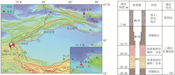
图 1 新10井构造环境(a)及其井孔结构(b)图
F1:柴窝堡盆地南缘断裂;F2:红雁池断裂;F3:雅玛克里断裂;F4:西山断裂;F5:二道沟断裂;F6:阜康断裂; F7:兴地断裂;F8:柯坪断裂;F9:西昆仑北缘断裂;F10:布伦口断裂
Figure 1. Geotectonic environment (a) and borehole structure (b) of Xin10 well
F1: Southern margin fault of Chaiwopu basin; F2: Hongyanchi fault; F3: Yama-Kerrey fault; F4: Xishan fault; F5: Erdaogou fault; F6: Fukang fault; F7: Xingdi fault; F8: Kalpin fault; F9: Northern margin fault of West Kunlun; F10: Bulunkou fault
![]()
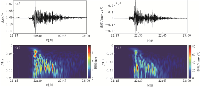
图 2 新10井水震波(左)与水磨沟台地震波(右)的形态(a, b)及时频特征(c, d)对比
Figure 2. Waveforms (a, b) and time-frequency characteristics (c, d) of hydroseismogram in the Xin10 well (left) and those of the seismic waves in Shuimogou station (right)
![]()
图 3 时间域水位与地表运动速度垂向分量的幅度对比
(a)水位与垂向速度散点图; (b)不同周期τ的水位幅值变化; (c)不同周期τ的垂向速度变化; (d)不同周期τ的水位与垂向速度振幅比m
Figure 3. Amplitude comparison between water level and vertical component of ground motion velocity in time domain
(a) Scatter diagram of water level versus vertical velocity; (b) Amplitude of water level in different periods τ; (c) Vertical velocity changes in different periods τ; (d) Amplitude ratio m of water level to vertical velocity in different periods τ
![]()
图 4 水位(a)与地表运动速度垂向分量(b)的频谱对比
Figure 4. Spectrum comparison between water level (a) and vertical component of ground motion velocity (b)
![]()
图 5 频率域水位与地表运动速度垂向分量的散点图(a)及其振幅比m (b)
Figure 5. Scatter diagram (a) and amplitude ratio m (b) of water level to vertical component of ground motion velocity in frequency domain
![]()
图 6 水震波变化幅值比R (a)和放大因子比R′ (b)
Figure 6. Amplitude ratio R of water level changes (a) and amplification factor ratio R′ (b) of hydroseismogram
![]()
图 7 不同渗透系数K下新10井水震波放大因子的理论值和实测值
(a)水位对含水层孔隙压力波动的放大因子A; (b)水位对地表垂向位移的放大因子A′
Figure 7. Theoretical values and measured values of amplification factor for the Xin10 well under different permeability coefficients K
(a) Amplification factor A of water level fluctuation to aquifer pore pressure; (b) Amplification factor A′ of water level to vertical displacement of ground surface
-
刘序俨, 郑小菁, 王林, 季颖锋. 2009.承压井水位观测系统对体应变的响应机制分析[J].地球物理学报, 52(12): 3147-3157. doi: 10.3969/j.issn.0001-5733.2009.12.025. Liu X Y, Zheng X J, Wang L, Ji Y F. 2009. Response analysis of the well-water-level system in confined aquifer[J]. Chinese Journal of Geophysics, 52(12): 3147-3157. doi: 10.3969/j.issn.0001-5733.2009.12.025 (in Chinese).
舒优良, 张世民, 黄辅琼. 2006.印尼8.7级和8.5级两次强震周至深井的震时效应研究[J].地震地磁观测与研究, 27(2): 16-22. http://www.cnki.com.cn/Article/CJFDTotal-FZJS200502015.htm Shu Y L, Zhang S M, Huang F Q. 2006. A study on earthquake-time effect of Zhouzhi deep borehole on two strong earthquakes: Magnitude 8.7 and magnitude 8.5 in Indonesia[J]. Seismological and Geomagnetic Observation and Research, 27(2): 16-22 (in Chinese). doi: 10.1007/s11589-009-0149-4
舒优良, 张世民, 黄辅琼. 2014.汶川8.0级地震周至深井水震波的记录特征[J].震灾防御技术, 9(增刊): 572-580. http://kns.cnki.net/KCMS/detail/detail.aspx?filename=zzfy2014s1002&dbname=CJFD&dbcode=CJFQ Shu Y L, Zhang S M, Huang F Q. 2014. Characteristics of water level depth vibration of Zhouzhi deep well during Wenchuan M8.0 earthquake[J]. Technology for Earthquake Disaster Prevention, 9(S): 572-580 (in Chinese). https://www.sciencedirect.com/science/article/pii/S0040195116304905
Barbour A J. 2015. Pore pressure sensitivities to dynamic strains: Observations in active tectonic regions[J]. J Geophys Res, 120(8): 5863-5883. doi: 10.1002/2015JB012201
Blanchard F B, Byerly P. 1935. A study of a well gauge as a seismograph[J]. Bull Seismol Soc Am, 25(40): 313-321. http://bssa.geoscienceworld.org/content/25/4/313
Brodsky E E, Roeloffs E A, Woodcock D, Gall I, Manga M. 2003. A mechanism for sustained groundwater pressure changes induced by distant earthquakes[J]. J Geophys Res, 108(B8): 2390. doi: 10.1029/2002JB002321.
Cooper Jr H H, Bredehoeft J D, Papadopulos I S, Bennett R R. 1965. The response of well-aquifer systems to seismic waves[J]. J Geophys Res, 70(16): 3915-3926. doi: 10.1029/JZ070i016p03915.
Eaton J P, Takasaki K J. 1959. Seismological interpretation of earthquake-induced water-level fluctuations in wells[J]. Bull Seismol Soc Am, 49(3): 227-245. http://bssa.geoscienceworld.org/content/49/3/227
Elkhoury J E, Brodsky E E, Agnew D C. 2006. Seismic waves increase permeability[J]. Nature, 441(7097): 1135-1138. doi: 10.1038/nature04798.
Elkhoury J E, Niemeijer A, Brodsky E E, Marone C. 2011. Laboratory observations of permeability enhancement by fluid pressure oscillation of in situ fractured rock[J]. J Geophys Res, 116(B2): B02311. doi: 10.1029/2010JB007759.
He A H, Fan X F, Zhao G, Liu Y, Singh R P, Hu Y L. 2017. Co-seismic response of water level in the Jingle well (China) associated with the Gorkha Nepal (MW7.8) earthquake[J]. Tectonophysics, 714/715: 82-89. doi: 10.1016/j.tecto.2016.08.019.
Hsieh P A, Bredehoeft J D, Farr J M. 1987. Determination of aquifer transmissivity from earth tide analysis[J]. Water Resour Res, 23(10): 1824-1832. doi: 10.1029/WR023i010p01824
Liu L B, Roeloffs E, Zheng X Y. 1989. Seismically induced water level fluctuations in the Wali well, Beijing, China[J]. J Geophys Res, 94(B7): 9453-9462. doi: 10.1029/JB094iB07p09453.
Ma Y C, Huang F Q. 2017. Coseismic water level changes induced by two distant earthquakes in multiple wells of the Chinese mainland[J]. Tectonophysics, 694: 57-68. doi: 10.1016/j.tecto.2016.11.040
Manga M, Beresnev I, Brodsky E E, Elkhoury J E, Elsworth D, Ingebritsen S E, Mays D C, Wang C Y. 2012. Changes in permeability caused by transient stresses: Field observations, experiments, and mechanisms[J]. Rev Geophys, 50(2): RG2004. doi: 10.1029/2011RG000382.
Manga M, Wang C Y, Shirzaei M. 2016. Increased stream discharge after the 3 September 2016 MW5.8 Pawnee, Oklahoma earthquake[J]. Geophys Res Lett, 43(22): 11588-11594. doi: 10.1002/2016GL071268.
Mays D C. 2010. Contrasting clogging in granular media filters, soils, and dead-end membranes[J]. J Environ Eng, 136(5): 475-480. doi: 10.1061/(ASCE)EE.1943-7870.0000173.
Montgomery D R, Manga M. 2003. Streamflow and water well responses to earthquakes[J]. Science, 300: 2047-2049. doi: 10.1126/science.1082980.
Pride S R, Berryman J G, Harris J M. 2004. Seismic attenuation due to wave-induced flow[J]. J Geophys Res, 109(B1): B01201. doi: 10.1029/2003JB002639.
Rexin E E, Oliver J, Prentiss D. 1962. Seismically-induced fluctuations of the water level in the Nunn-Bush Well in Milwaukee[J]. Bull Seismol Soc Am, 52(1): 17-25. https://pubs.geoscienceworld.org/ssa/bssa/article-abstract/52/1/17/101282/seismically-induced-fluctuations-of-the-water?redirectedFrom=fulltext
Shalev E, Kurzon I, Doan M L, Lyakhovsky V. 2015. Water-level oscillations caused by volumetric and deviatoric dynamic strains[J]. Geophys J Int, 204(2): 841-851. http://adsabs.harvard.edu/abs/2016GeoJI.204..841S
Shi Z, Wang G, Manga M, Wang C Y. 2015. Continental-scale water-level response to a large earthquake[J]. Geofluids, 15(1/2): 310-320. doi: 10.1111/gfl.12099/abstract
Shih D C F, Wu Y M, Chang C H. 2013. Significant coherence for groundwater and Rayleigh waves: Evidence in spectral response of groundwater level in Taiwan using 2011 Tohoku earthquake, Japan[J]. J Hydrol, 486: 57-70. doi: 10.1016/j.jhydrol.2013.01.013
Stockwell R G, Mansinha L, Lowe R P. 1996. Localization of the complex spectrum: The S transform[J]. IEEE Trans Signal Process, 44(4): 998-1001. doi: 10.1109/78.492555
Sun X L, Wang G C, Yang X H. 2015. Coseismic response of water level in Changping well, China, to the MW9.0 Tohoku earthquake[J]. J Hydrol, 531: 1028-1039. doi: 10.1016/j.jhydrol.2015.11.005
Wang C Y, Wang C H, Manga M. 2004. Coseismic release of water from mountains: Evidence from the 1999 (MW7.5) Chi-Chi, Taiwan, earthquake[J]. Geology, 32(9): 769-772. doi: 10.1130/G20753.1.
Weingarten M, Ge S M. 2014. Insights into water level response to seismic waves: A 24 year high-fidelity record of global seismicity at Devils Hole[J]. Geophys Res Lett, 41(1): 74-80. doi: 10.1002/2013GL058418
Yan R, Woith H, Wang R J. 2014. Groundwater level changes induced by the 2011 Tohoku earthquake in China mainland[J]. Geophys J Int, 199(1): 533-548. doi: 10.1093/gji/ggu196
Yan R, Wang G C, Shi Z M. 2016. Sensitivity of hydraulic properties to dynamic strain within a fault damage zone[J]. J Hydrol, 543: 721-728. doi: 10.1016/j.jhydrol.2016.10.043
Zhang Y, Fu L Y, Huang F Q, Chen X Z. 2015. Coseismic water-level changes in a well induced by teleseismic waves from three large earthquakes[J]. Tectonophysics, 651: 232-241. https://www.sciencedirect.com/science/article/pii/S004019511500195X
-
期刊类型引用(9)
1. 贾永斌,闫玮,祖丽皮牙·艾尼瓦尔,汪成国. 乌什M_S7.1地震引起新55井、新46井水位水温同震响应分析. 内陆地震. 2024(02): 158-165 .  百度学术
百度学术
2. 梁卉,高小其,颜龙. 2023年2月6日土耳其两次7.8级地震引起的井水位同震响应对比分析. 地震. 2024(03): 96-107 . 百度学术
3. 洪旭瑜,陈祥开,秦双龙,林加宝. M_S≥6.0地震引起的永安井水位同震响应特征研究. 华南地震. 2023(03): 39-45 . 百度学术
4. 毛巍颖. 云南思茅大寨井与大理月溪井水位同震响应对比分析. 华南地震. 2022(01): 31-37 . 百度学术
5. 孙小龙,刘耀炜,付虹,晏锐. 我国地震地下流体学科分析预报研究进展回顾. 地震研究. 2020(02): 216-231+417 . 百度学术
6. 赵頔,张宝匀,丁谋谋,孙云山. 北京昌平井水位对日本M_W9.0地震的响应. 内陆地震. 2020(04): 347-354 . 百度学术
7. 方震,黄显良,汪小厉,杨源源,倪红玉,张彬. 庐江地热温泉1号井水氡远场强震震后效应及机理分析. 地震学报. 2020(06): 732-744+782 . 本站查看
8. 陆丽娜,李静,薛红盼,汪啸,张雷,王建. 赵各庄井地下流体的映震响应. 震灾防御技术. 2019(01): 174-190 . 百度学术
9. 崔瑾,丁风和,曾宪伟,司学芸. 宁夏井水位观测同震响应特征研究及机理探讨. 地球物理学进展. 2019(04): 1281-1287 . 百度学术
其他类型引用(3)

 下载:
下载:


计量
- 文章访问数: 1412
- HTML全文浏览量: 668
- PDF下载量: 45
- 被引次数: 12
